Excel's ability to freeze rows and columns is crucial for navigating and analyzing extensive spreadsheets. By keeping headers or key identifiers visible while scrolling, users maintain context and boost efficiency. Whether you call it "freezing" or "pinning," mastering this feature is essential for anyone working with complex data.
All Steps for Freezing a Row in Excel Sheet
Freezing rows and columns in Excel is crucial for maintaining key data, such as header rows, visible when scrolling through large datasets. It ensures you can always refer to column titles or other vital information, improving navigation and data accuracy.
1. Select Row Below: Click on the row number directly below the row you want to freeze. (e.g., to freeze row 1, click on row 2).
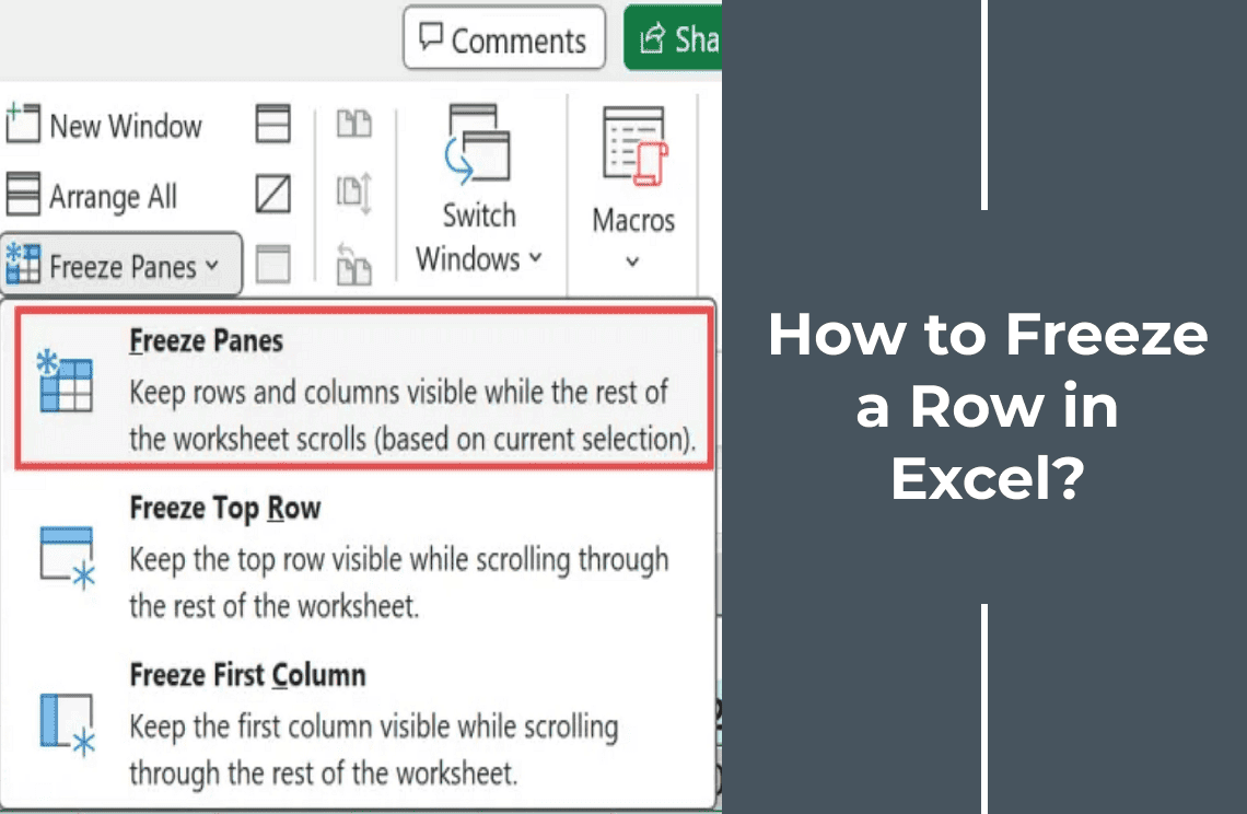
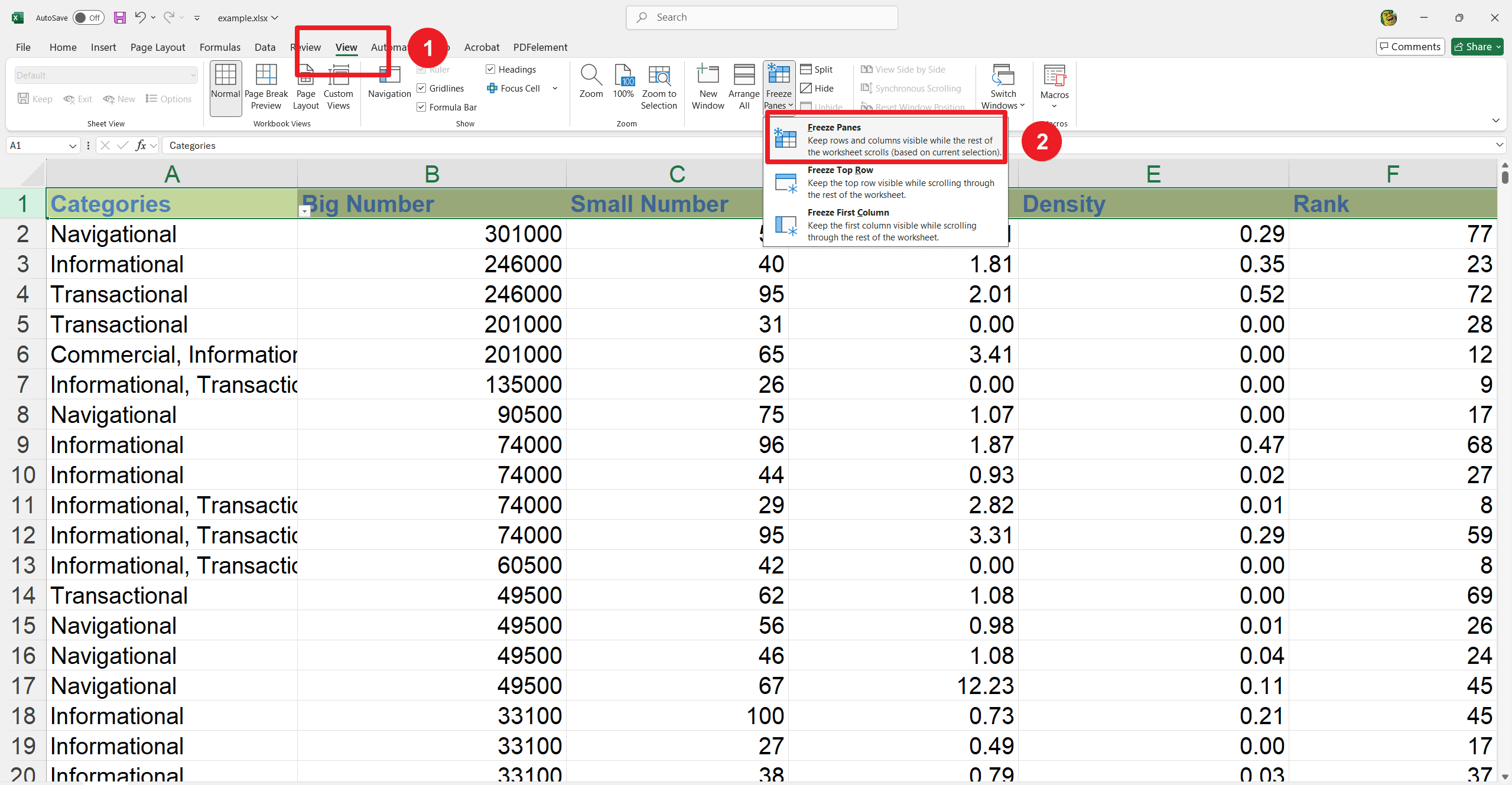
2. Freeze Panes: Go to the "View" tab, click "Freeze Panes," and then select "Freeze Panes."
3. Verify Freezing: A gray line will appear, indicating the frozen area. Now, when you scroll, the rows above the line will stay visible.
Steps for Freezing the Top Row
For simpler spreadsheets, quickly freezing the top row or first column can be easily done with these steps:
Use the Freeze Panes Command
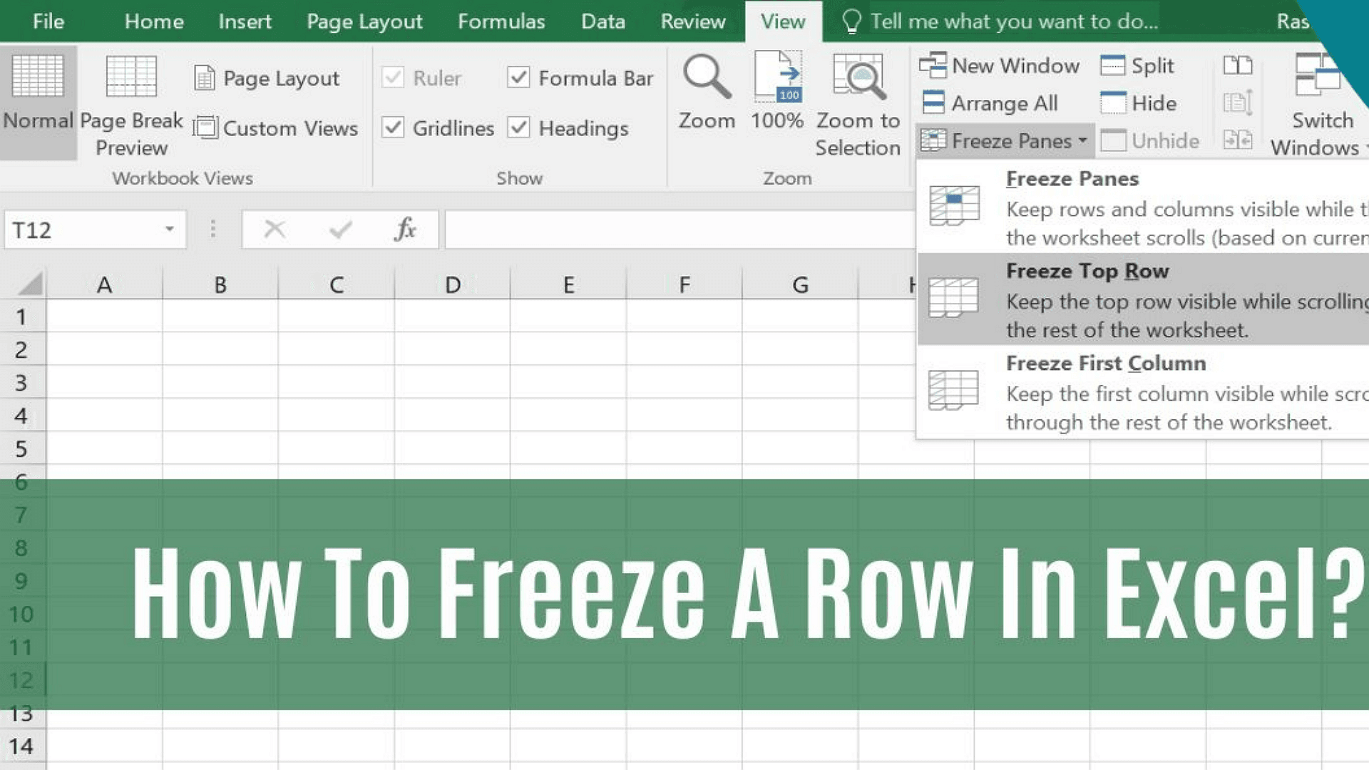
1. Click to the View tab. It is found on the Ribbon at the top of the Excel window.
2. Select the Freeze Panes dropdown: Click on the dropdown to view available options.
3. Choose "Freeze Top Row": This will lock the topmost row in place.
4. Select "Freeze First Column" to freeze the first column instead.
These steps ensure critical headers or key data remain visible, streamlining data management and analysis.
Steps to Unfreeze Panes
Do you need to unfreeze panes in Excel to reset your view options sometimes? Now you can reapply the freeze to a different row or column. You can also view your data without any frozen rows or columns.
Unfreeze Panes Command
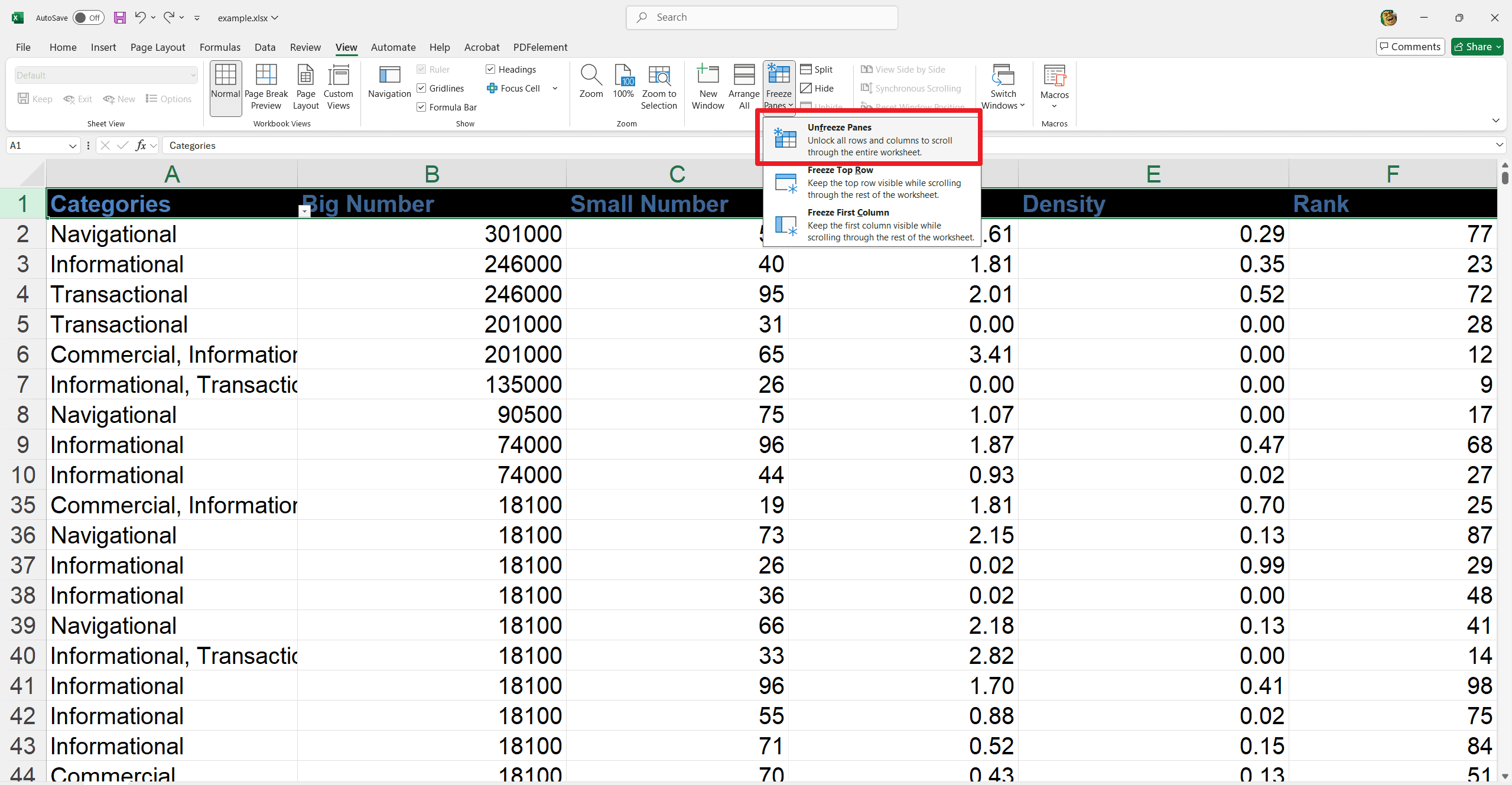
1. Go to the View tab: It is located on the Ribbon at the Excel window’s top.
2. Choose the Freeze Panes dropdown: Now click the dropdown menu to reveal options in it.
3. Select Unfreeze Panes to remove any frozen rows or columns. You can reapply the freeze to new rows or columns as needed by unfreezing panes. It allows greater flexibility in managing your spreadsheet's outlook.
How to Freeze a Row in Excel Using Mobile?
You can also freeze rows in the Microsoft Excel app on iOS or Android by following these simple steps:
1. Open Your File: Launch the Excel app and open the spreadsheet.
2. Go to View: Tap "Home" (or "View") and then "View."

3. Freeze Top Row/First Column: Select "Freeze Top Row" or "Freeze First Column" to lock the respective area.

4. Unfreeze: Tap "Freeze Top Row" (or "Freeze First Column") again to remove the freeze.
Freeze Multiple Rows or Columns
To freeze multiple rows or columns in Excel, follow these steps:
Selecting Rows or Columns
- Select the Row or Column:
- For multiple rows, tap the row number immediately after the last row you want to freeze.
- For multiple columns, tap the column letter immediately after the last column you want to freeze.
Apply Freeze Panes
- Tap "View": Navigate to the View settings.
- Tap "Freeze Panes":
- It will freeze all rows above and columns to the left of your selection.
Unfreeze Panes
Simply tap Freeze Panes again to unfreeze. It will remove the checkmark and unfreeze the panes.
It allows you to lock in multiple rows or columns for better navigation and data management in your Excel workbook.
Additional Viewing Options in Excel
Opening a New Window
- Navigate to the View tab.
- Click "New Window": This opens another window of the same workbook.
- Arrange the windows by clicking "Arrange All."
Example Scenarios
- Compare data side by side.
- Monitor different sheets simultaneously.
- Splitting Worksheet Panes
Instructions
- Choose the cell where you want to split the worksheet.
- Go to the View tab.
- Tap on the Split command to divide the worksheet into four panes.
- Drag the dividers to create the desired custom comparison views.
Use Case Example
- Splitting panes allow for simultaneous viewing and comparing data from different sections of a large worksheet, enhancing analysis and navigation efficiency.
Shortcuts
- Go to the Quick Access Toolbar
- Tap on the small dropdown arrow
- Choose More Commands
- See the Choose commands button from dropdown
- Choose All Commands
- Now Scroll down to Freeze Panes
- Tap on it
- Now Click Add button
- Apply your changes by clicking OK
For Further Reading
Freezing and unfreezing Excel rows and columns offer significant data management benefits. These features allow you to keep crucial information in view while scrolling through large datasets, enhancing your ability to analyze and interpret data effectively. Additionally, splitting panes facilitates the simultaneous comparison of different worksheet sections. Utilizing these powerful tools can streamline your workflow, maintain focus on key data, and improve overall productivity. We encourage you to explore these features in your worksheets to experience their benefits firsthand and optimize your Excel usage.
For more great tips and tools to improve your Excel skills, I highly recommend visiting the following resources:
These blogs and How-to sections offer a wealth of information. It includes practical advice and detailed guides that maximize working with Excel and other tools. So, feel free to explore these resources to enhance your knowledge and skills further!

