Do you need to learn basic Excel functions? Because, they are essential for anyone with data analysis and handling. These skills can improve efficiency and accuracy in students, business professionals and all others involved in any data-driven field. So, this guide will explore how to sum, average, and analyze data within Excel columns easily. Yes, you will understand these fundamental techniques to manage your data more effectively by the end of learning these methods.
How to Sum a Column in Excel?
Understanding AutoSum
The AutoSum tool in Excel is a simple yet powerful feature for quickly adding values to a column. It automatically identifies the range of numbers you want to sum and inserts the appropriate SUM formula. Here is a quick guide on using AutoSum for a single column:
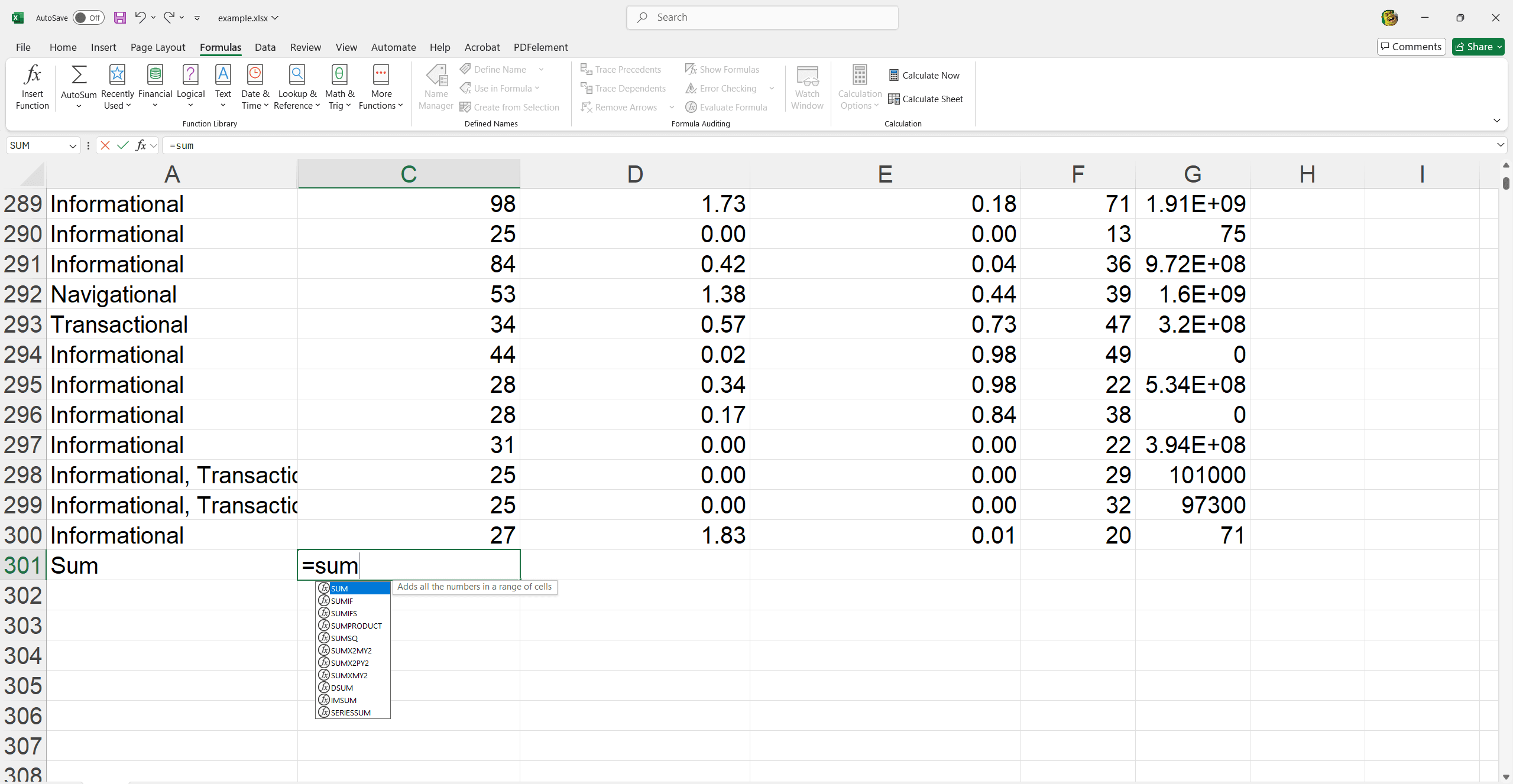
1. Select the cell directly below the column of numbers you want to sum.
2. Navigate to the Formula tab on the Ribbon.
3. Click on the AutoSum button (Σ symbol).
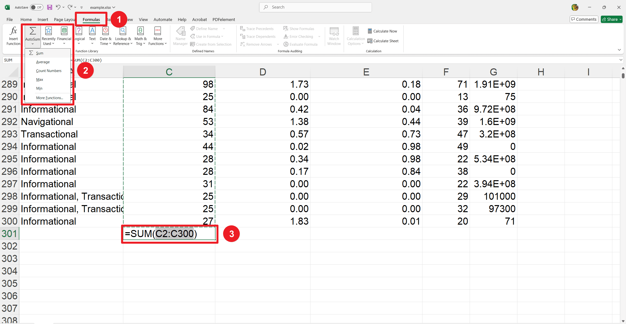
4. See the Drop down menu and click on Sum.
5. Press Enter to confirm.
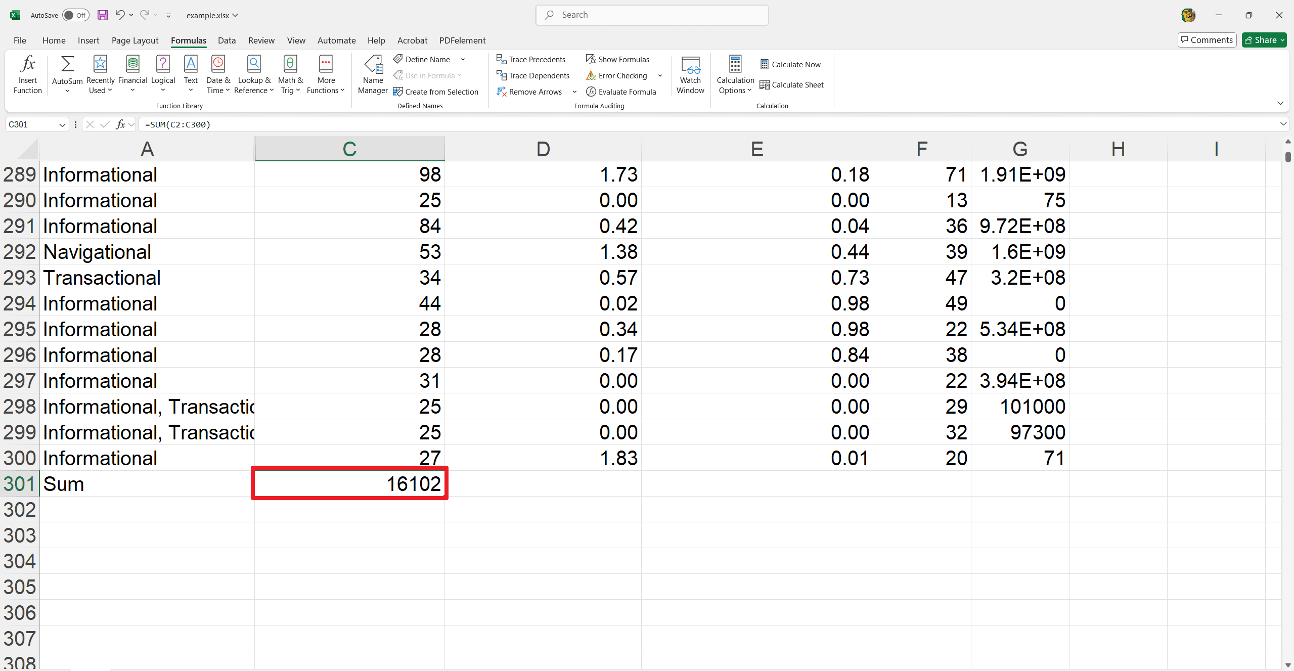
Your selected cell will now display the total sum of the column values above it.
Using the SUM Function
This function allows you to add values from one or multiple columns manually. However, it is useful when you want to specify a range of cells particularly. See how to use the SUM function in this procedure:
1. Click on the cell where you want the total to appear.
2. Type "=SUM(".
3. Choose the range of cells you want to add by clicking and dragging or typing the cell range. Close the bracket by typing “)”. Then, Press Enter to see the result.
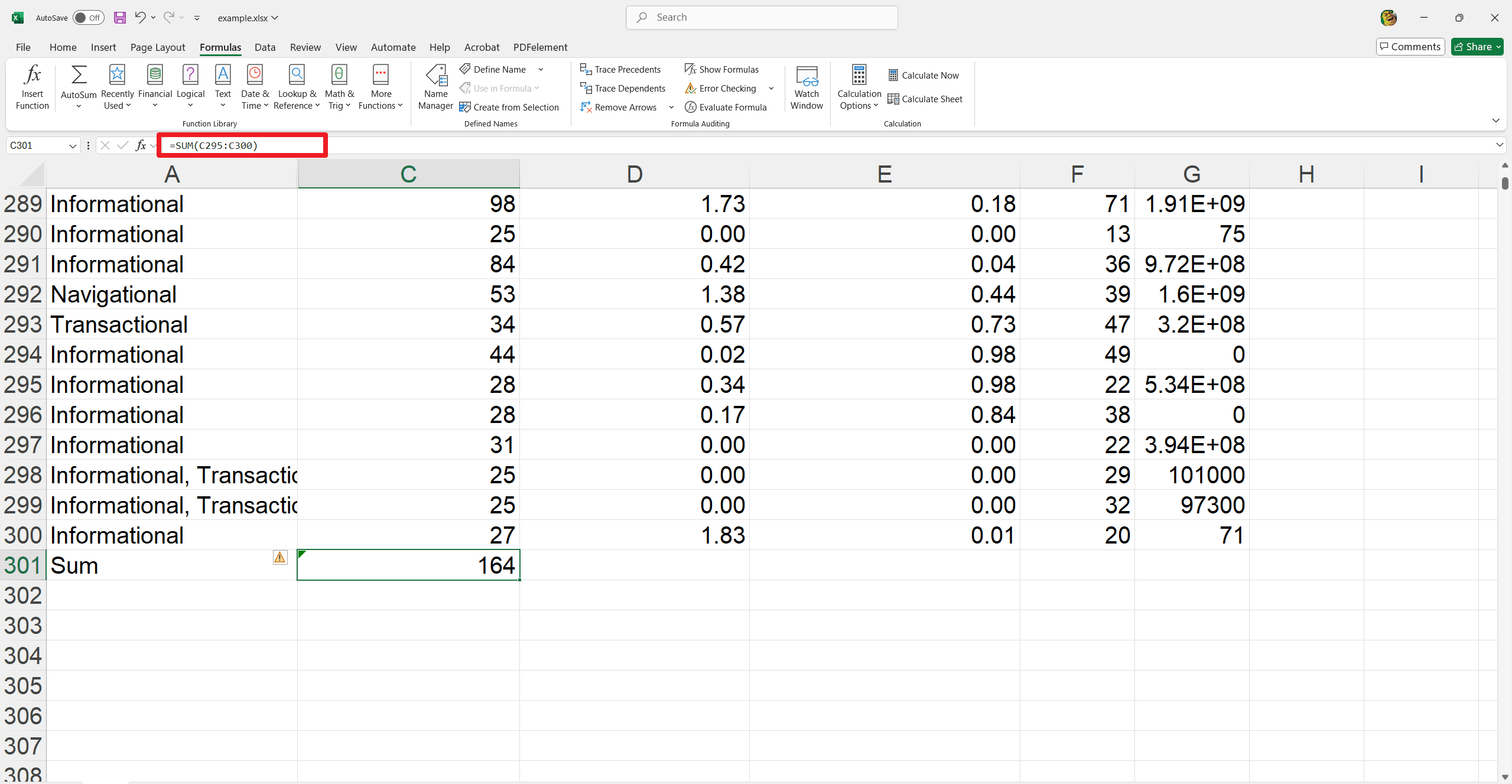
It will give you the total sum for your specified cell range.
Advanced Summing with SUMIF
The SUMIF function allows you to sum column values based on specific criteria conditionally. It is useful for summing only the values that meet certain conditions. Here is how to use SUMIF:
1. Click on the cell where you want the total to appear.
2. Type "=SUMIF(".
3. Enter the range of cells to evaluate for criteria (e.g., B2:B10).
4. Type a comma and specify the criteria (e.g., ">10" for values greater than 10 or "Completed" for text criteria).
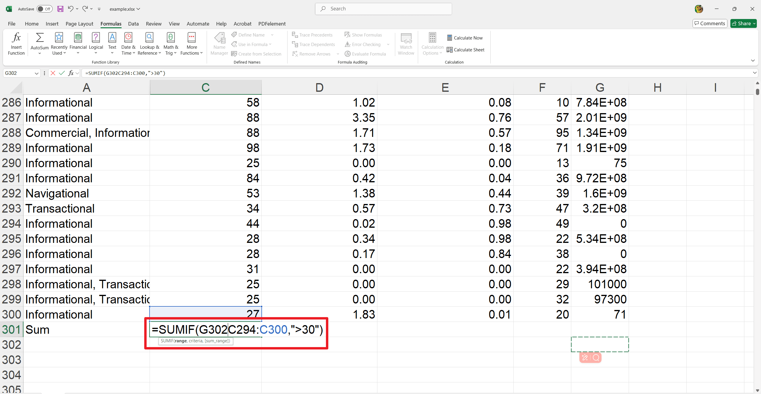
5. Type another comma and enter the range of cells to sum.
6. Close the bracket by typing ")" and press Enter.
For example, =SUMIF(A1:A10, ">10", B1:B10) sums values in B1:B10 where corresponding A1:A10 values are greater than 10.
Quick Totals with the Status Bar
The Status Bar in Excel provides a convenient way to see the sum of selected column values without formula input. It gives quick insights and is especially useful for calculations on the fly. Here is how to use it:
1. Select the range of cells in the column you want to sum.
2. Look at the bottom-right corner of the Excel window, where the Status Bar is located.
3. The Status Bar automatically displays the sum of the selected cells, along with other calculations like average and count.
It allows you to quickly monitor totals without altering your spreadsheet.
How to Average Data in Excel Columns?
The AVERAGE Function
The AVERAGE function in Excel simplifies finding the mean of column data. This function calculates the average of the selected range of values. Here is how to use it:
1. Select the cell where you want the average to appear.
2. Type "=AVERAGE(".
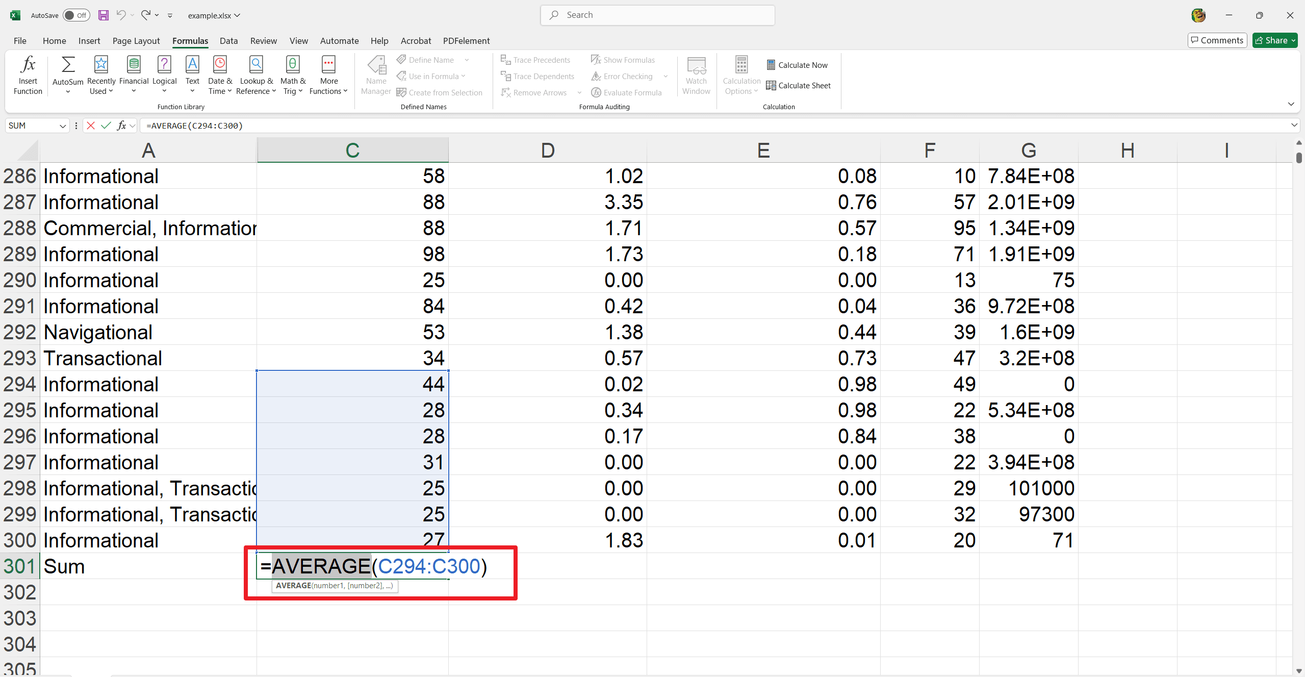
3. Highlight the range of cells you want to average, or type the cell range.
4. Close the bracket by typing ")".
5. Press Enter to see the result.
For example, =AVERAGE(A1:A10) calculates the average values in cells A1 to A10 and shows the mean of the selected data range.
Using AVERAGEIF for Conditional Averages
This function calculates the average of cells that meet specified criteria. It makes easy to find conditional averages in your figures. See the procedure:
1. Select the cell where you want the conditional average to appear
2. Type "=AVERAGEIF(".
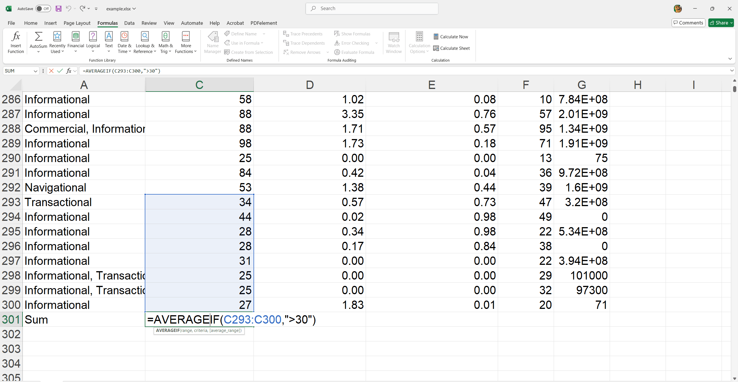
3. Enter the range of cells to evaluate.
4. Type a comma, then specify the criteria (e.g., ">B2:B6" for values greater than 20 or "Active" for text criteria).
5. Close the bracket by typing ")".
6. Press Enter to see the result.
For example, =AVERAGEIF(A1:A10, ">20") calculates the average of values in cells A1 to A10 that are greater than 100.
How to Analyze Data in Excel?
Creating Data Tables
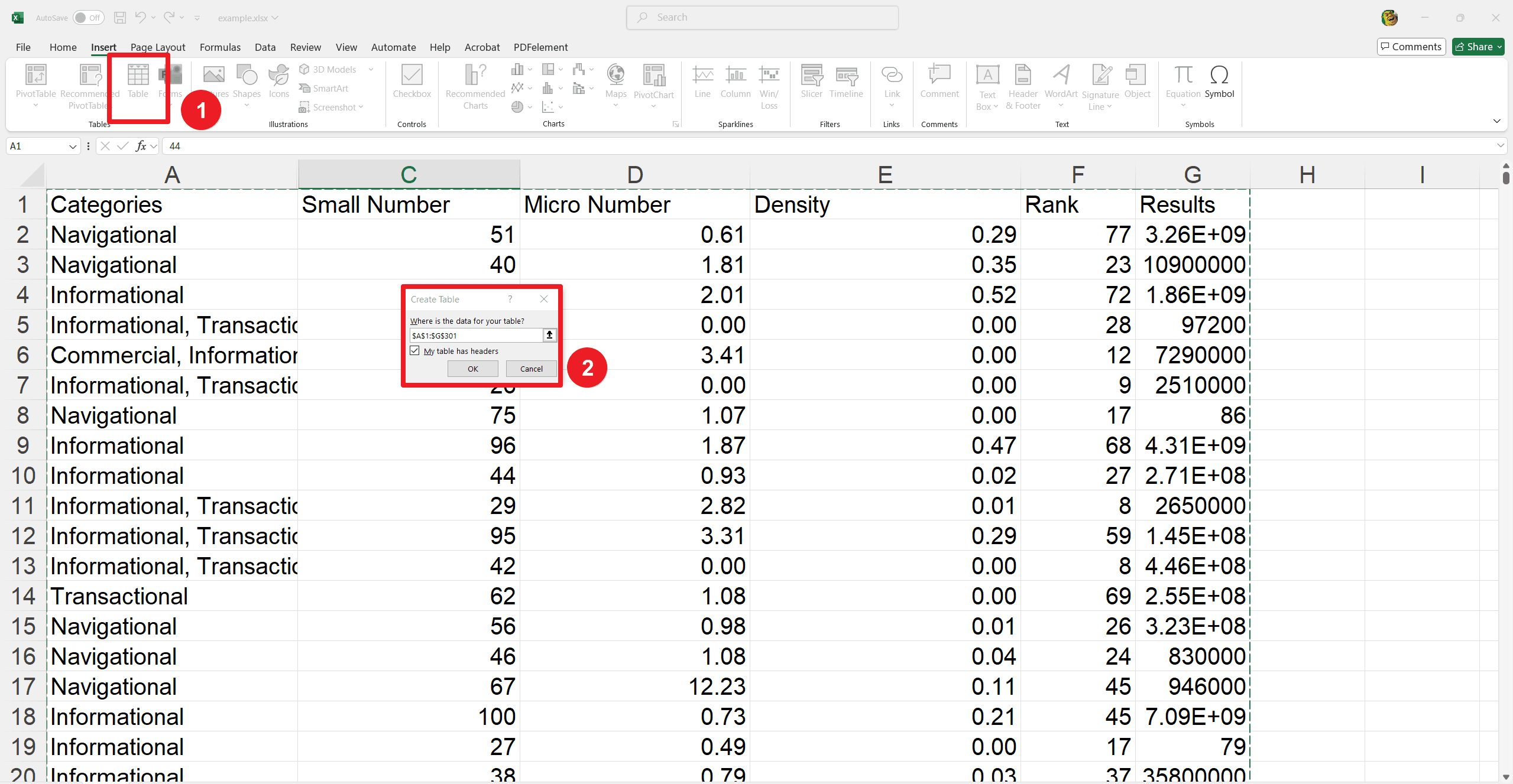
Transforming datasets into tables in Excel enhances analysis and allows for dynamic data ranges. Here's how to create a data table and use a total row for comprehensive insights:
1. Select your dataset (including headers).
2. Go to the Insert tab and click Table.
3. Ensure "My table has headers" is checked, then click OK.
To enable a total row:
1. Click anywhere in the table.
2. Go to the Table Design tab.
3. Check the Total Row box.
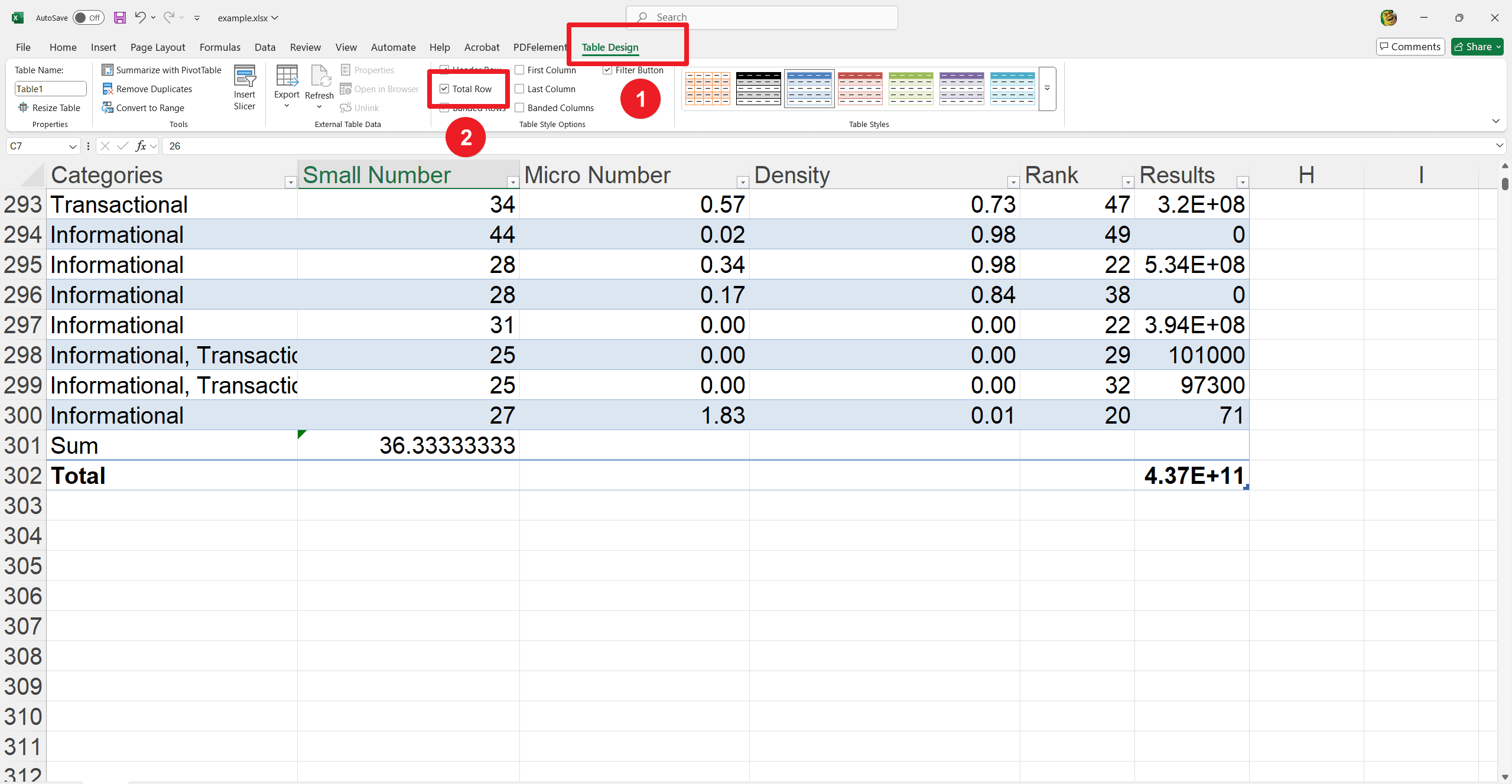
The total row will appear at the bottom of the table, where you can click cells to display sums, averages, counts, and more for each column.
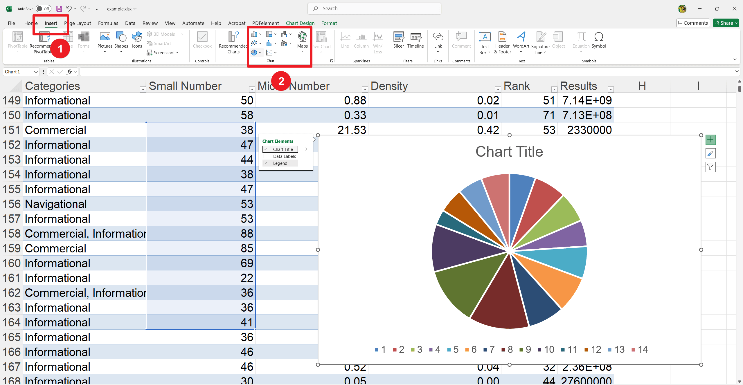
Visual Analysis with Charts and Graphs
Converting tabulated data into charts enhances visual comprehension and makes identifying patterns stress free. However, charts can provide quick insights for making data interpretation artless.
To generate and customize a column chart:
1. Highlight the data range you want to visualize (including headers).
2. Go to the Insert tab.
3. Click on the Column Chart icon and select a desired chart style (e.g., clustered column).
4. The chart will appear on your spreadsheet.
To customize:
1. Click on the chart to access Chart Tools.
2. Use the Design and Format tabs to modify chart elements such as colors, labels, and titles for better presentation and clarity.
Few Excel Shortcuts
Excel shortcuts can significantly enhance workflow efficiency, saving time and effort. Some valuable shortcuts include:
- Ctrl + C: Copy selected cells
- Ctrl + V: Paste the copied content
- Ctrl + Z: Undo the last action
- Ctrl + Y: Redo the last action
- Ctrl + Shift + L: Toggle filters on/off
- Alt + =: Automatically sum a column or row of numbers with AutoSum
- F2: Edit the active cell, allowing quick error corrections
These shortcuts streamline tasks and improve data analysis speed.
Maintain Data Integrity with Pro Tips
Ensuring data integrity is crucial when summing or analyzing data. Common errors include misaligned data and inconsistent formats, leading to incorrect outcomes. Here are some tips to maintain data consistency and accuracy:
- Consistent Formats: Ensure data is uniformly formatted. For example, dates should be entered consistently across the dataset.
- Avoid Blank Cells: Empty cells can skew analysis results. Use the IFERROR function to handle errors or fill in blanks with placeholders.
- Data Validation: Apply data validation rules to restrict input types and maintain data entry correctly.
- Regular Auditing: Review your data periodically for anomalies or discrepancies. It corrects errors on time.
- Backup Data: Backup your data regularly to prevent loss and maintain a reliable historical record for reference in future.
For Further Reading
This guide will explore essential Excel skills to sum, average, and analyze data competently. Mastering AutoSum and AVERAGEIF techniques and crafting insightful charts will be well on your way to becoming data analysis proficient.
Check out the Excel Tips and How-To and Tips at PDF Agile to deepen your knowledge and discover even more Excel secrets. They're great resources for continuing your journey. Practice and experiment with Excel's versatile features with these methods. The more you explore, the more powerful tools you will disclose. It is time to turn yourself into a data management pro!