The Pivot Table of Microsoft Excel is a powerful tool to convert raw data into actionable insight in data analysis. This guide provides a broad pivot table construction, manipulation, and use walkthrough, which makes users efficiently abbreviate, analyze, and imagine the complex dataset. From basic insertion and pruning to advanced filtering and summary calculation, this blog aims to demolish the process, allowing professionals to enhance the extended data-manufacturing decisions that can be enabled to take advantage of the Pivot tables.
Benefits and Uses of Pivot Tables:
- Data Summarization and Analysis: Pivot tables efficiently condense large datasets into meaningful summaries, facilitating rapid analysis and identification of trends. They enable data aggregation across multiple dimensions, providing a comprehensive overview of complex information.
- Enhanced Data Visualization: Pivot tables are the foundation for creating pivot charts visually representing data patterns and relationships. This graphical representation simplifies the interpretation of complex data, effectively communicating findings.
- Dynamic Data Exploration: Pivot tables offer interactive filtering and sorting capabilities, allowing users to dynamically explore data subsets. This flexibility enables targeted analysis and the identification of specific data points relevant to particular inquiries.
- Better Reporting: They automate the generation of summary reports. It significantly reduces the time and effort required for manual data handling. This automation enhances productivity and ensures consistency in reporting practices.
- Facilitation of Decision-Making: By providing clear and concise data summaries, pivot tables empower informed decision-making. They enable users to identify key performance indicators and assess the impact of various factors on business outcomes.
- Cross-Tabulation Analysis: Pivot tables allow for the easy creation of cross-tabulation reports, showing the relationship between two or more data sets. This is very useful for comparing data across multiple categories.
How to Insert a Pivot Table?
To insert a pivot table, adhere to the following procedure:
1. Choose any cell within the data range.
2. Go to the Insert tab on the Excel ribbon.
3. Select PivotTable within the Tables group
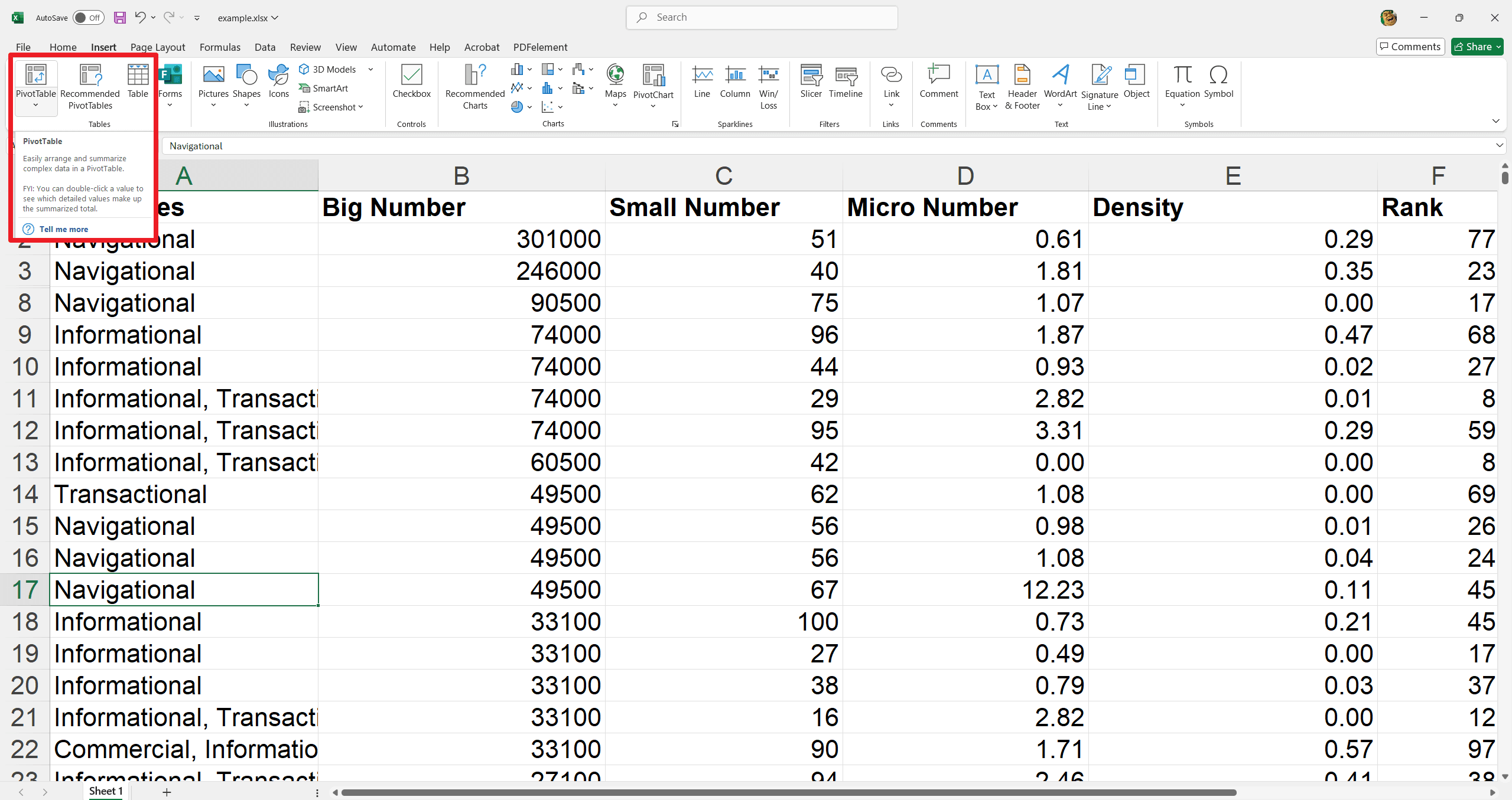
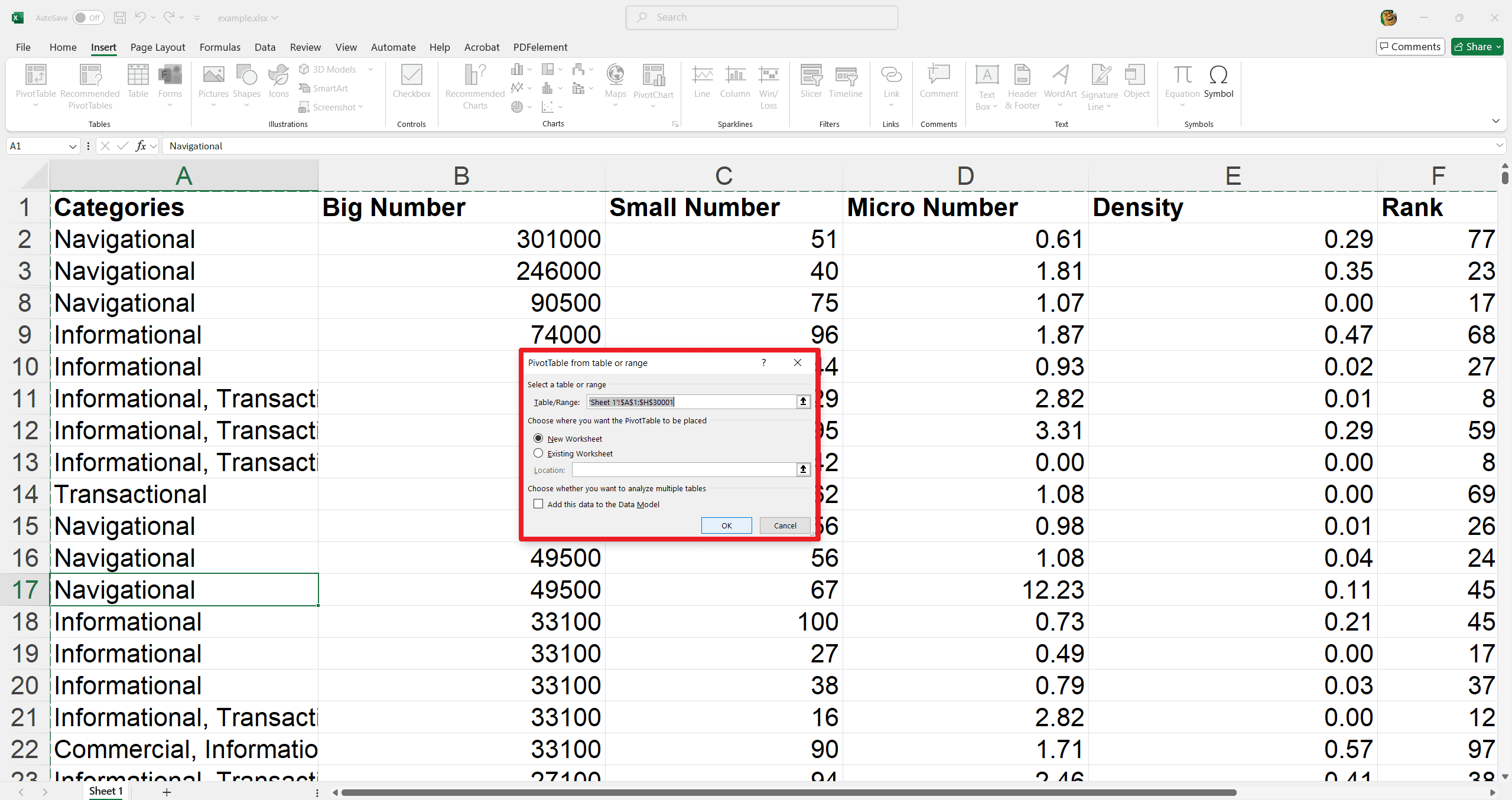
4. A dialog box will appear, wherein Excel automatically selects the data range.
5. The default placement for the pivot table is a "New Worksheet."
6. Confirm the selection by clicking "OK."
Drag Fields
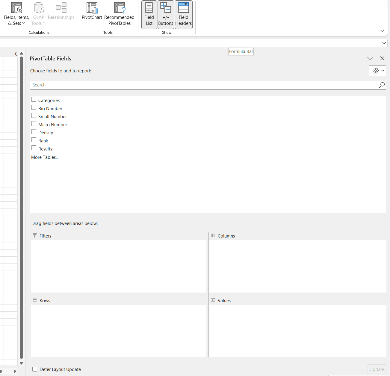
Pivot Table Fields pane will become obvious. Perform the following actions to generate the total exported amount for each product.
- Drag the "Category" field to the "Rows" area.
- Drag the "Big Number" field to the "Values" area.
- Drag the "Small Number" field and so forth to the "Filters" area.
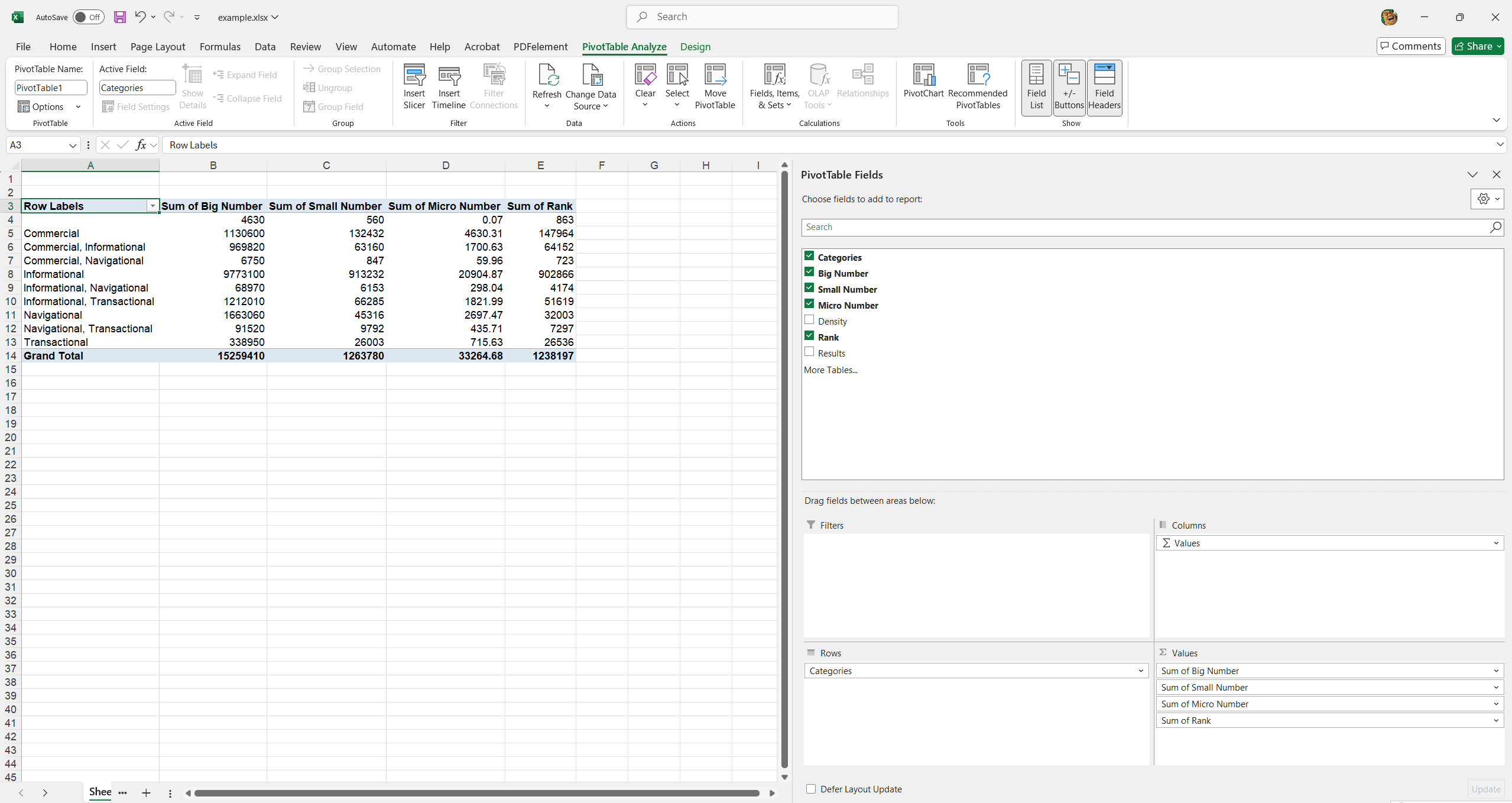
- The resulting pivot table will be displayed.
- Analysis of the table will demonstrate the primary export product.
How to Filter a Pivot Table?
Including the "Big Number" field in the "Filters" area enables filtering the pivot table by country. For example, to determine the highest exported products to France:
1. Click the filter dropdown menu.
2. Select "Big Number."
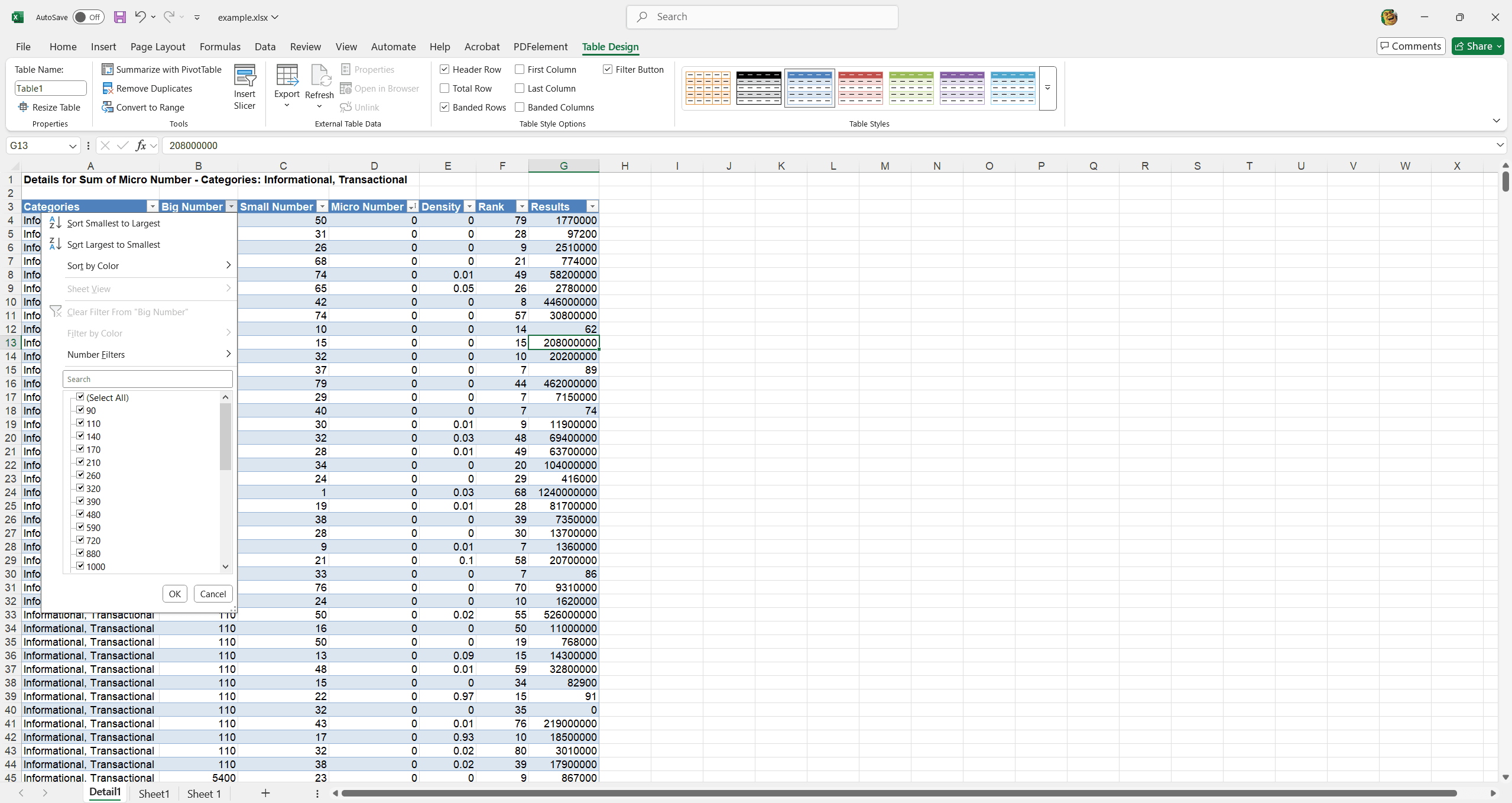
Result: The pivot table will display the exported amounts to France, highlighting the primary product.
Note: The standard filter (triangle adjacent to "Row Labels") can be utilized to display amounts for specific products exclusively.
How to Change Summary Calculation?
By default, Excel aggregates data through summation or item counting. To modify the calculation method, perform the following steps:
1. Select any cell within the "Sum of Small Number" column.
2. Right-click the selected cell.
3. Choose “Value Field Settings.”
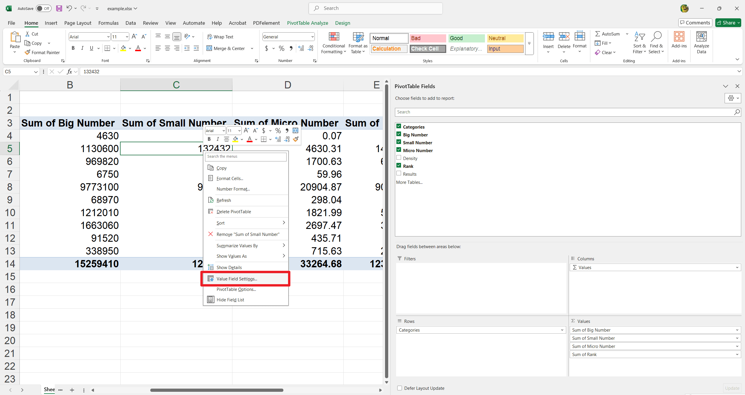
4. Select the desired calculation type. For instance, choose "Count."
5. Confirm the selection by clicking "OK."
Result: The pivot table will display the count of items, illustrating the frequency of specific product orders. For example, the output might show the number of "Apple" orders out of the total orders for a particular country.
Pivot Chart
To facilitate a straightforward comparison of numerical data, generate a pivot chart and apply a filter. While this may represent an advanced technique for some users, it demonstrates one of the many robust functionalities available within Excel's pivot table feature set.
How to Refresh a Pivot Table in Excel?
You need to refresh the pivot table to reflect any additions, modifications or deletions within the source figures. The quickest method is:
1. Right-click any cell within the pivot table.
2. Select “Refresh.”
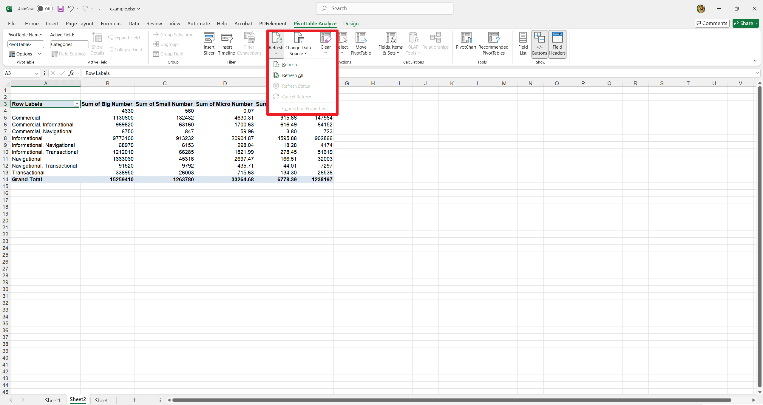
3. Alternatively, utilize the "PivotTable" tab:
- Tap in the pivot table to activate the PivotTable tab on the Excel ribbon.
- Now click the dropdown arrow next to Refresh All option.
- Select "Refresh All" to update all pivot tables within the workbook simultaneously.
- Select "Refresh" to update the currently selected pivot table.
4. By default, pivot tables do not automatically refresh. To enable automatic refresh upon file opening:
- Click within the pivot table to display the "PivotTable" tab.
- Click the "PivotTable" tab.
- Click "Settings".
PivotTable Settings pane will appear on the right side of the sheet.
- First scroll down and check the box next to Refresh data on file open option.
Final Words
With the power to master pivot tables within Excel, data analysis is significantly simplified. Summarization, filtering, and data visualization are accomplished with ease and speed, giving way to enhanced identification of vital trends and patterns and follow-up strategic actions. Whether sales data, financial statements, or any other complex dataset must be analyzed, pivot tables make extracting useful insights easily. With the steps outlined here, users can harness the feature's potential and elevate their data analysis game. If you want to learn more about PDF tutorials and Excel Tips, please check How-to & Tips | PDF Agile and Excel Tips | PDF Agile.

