Hello, Excel enthusiasts! If you've ever found yourself struggling with merging cells without losing valuable data, you're in the right place. Merging cells in Excel can be a lifesaver when organizing and presenting data neatly. In this blog, we're going to explore a handful of techniques that will help you become a pro at cell merging. Whether you're using functions like CONCATENATE, TEXTJOIN, or quick tricks with the ampersand symbol, I've got everything you need to master the art of merging cells.
How to Merge Cells in Excel in Windows?
Alright, let's dive right in and get those cells merged in Excel. It's a quick and easy process, so you'll be done in no time!
Step 1: First things first, go ahead and open Microsoft Excel. Make sure you have the worksheet open where you want to merge those cells.
Step 2: Now, select the adjacent cells you want to merge. You can do this by clicking and dragging to highlight multiple cells. Alternatively, you can hold down the Ctrl key and click each cell you want to include, one by one.
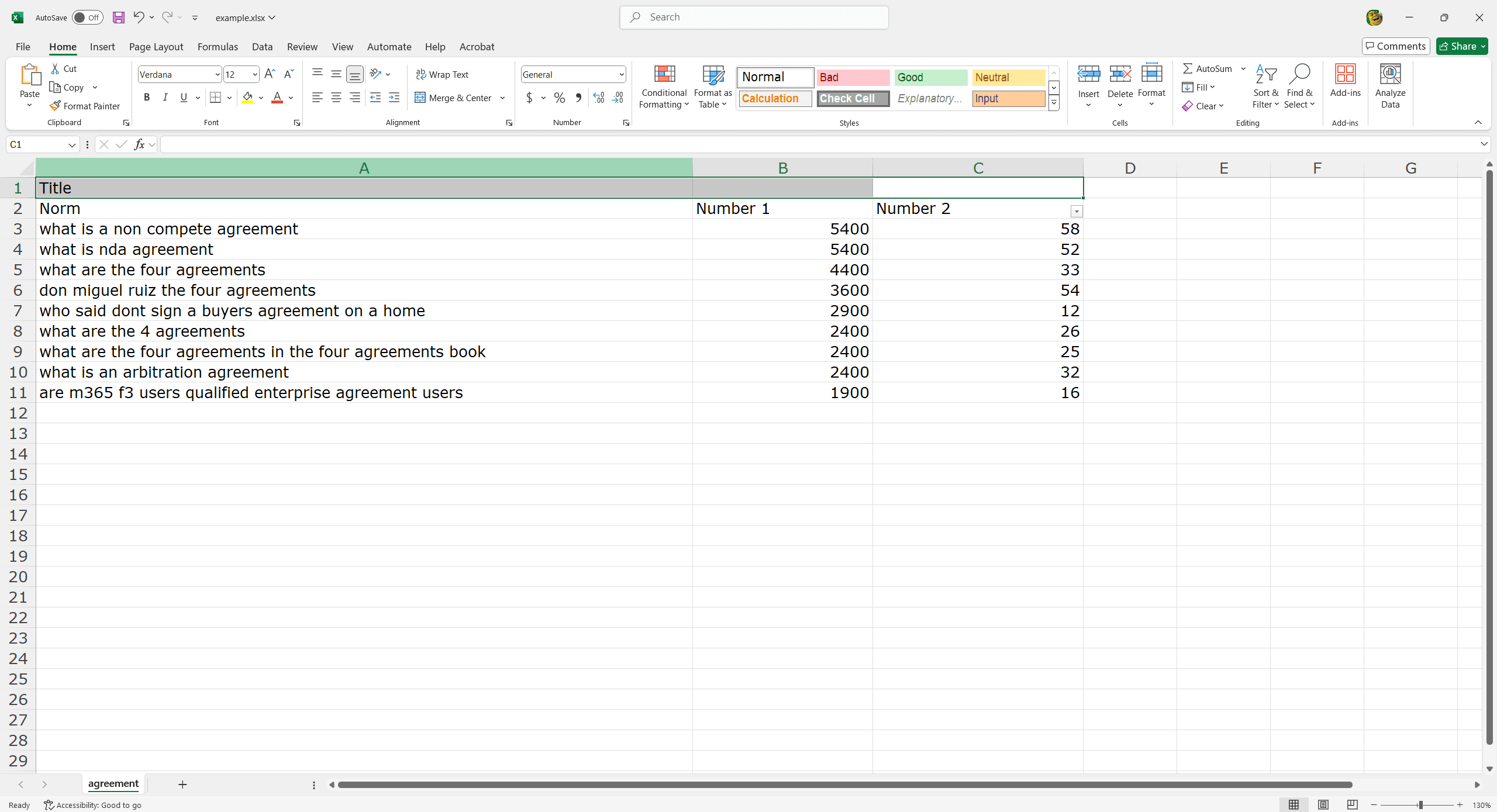
Step 3: Next, look up the Excel ribbon and find the Home tab.
Step 4: In the Home tab, head over to the Alignment group. There's a little dropdown arrow next to the Merge & Center button – go ahead and click that arrow.
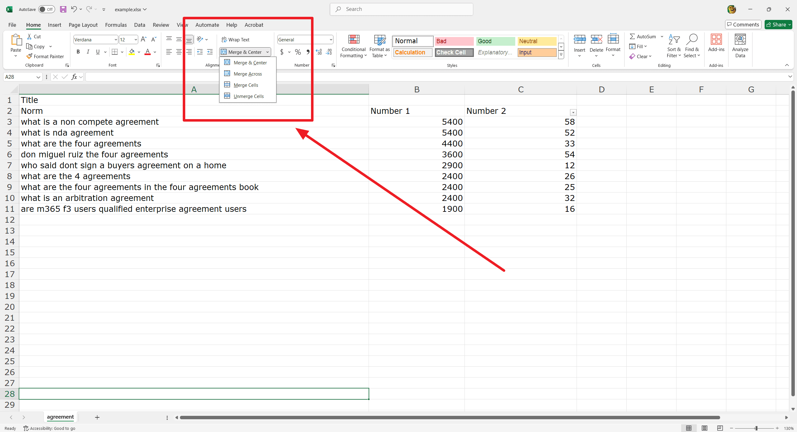
Step 5: From the dropdown menu, select the Merge Cells option.
At this point, you have a couple of choices:
- Merge & Center: This will merge your selected cells and center the content.
- Merge Across: This will merge cells within each row without centering the content.
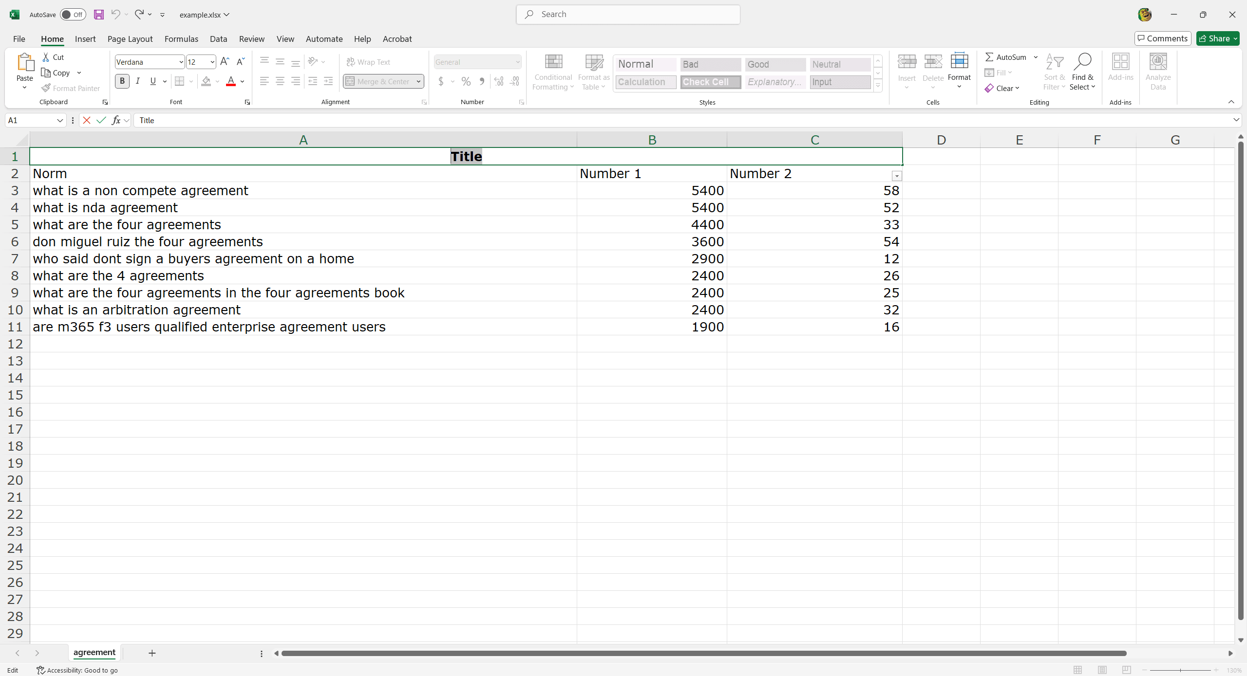
And just like that, the cells A1 and B1 are merged!
Quick Tip
Keep in mind this method only keeps the data in the leftmost cell (in this case, A1). If cells like B1 have data, be sure to move that data somewhere else before merging to avoid losing anything important.
There you go! It's really that simple. Happy merging!
Merging Cells on macOS
Here's a quick guide to merging cells in Excel on your Mac. It's simple and straightforward:
Step 1:
Start by opening your Excel worksheet. Once you're in, select the cells you're looking to merge.
Step 2:
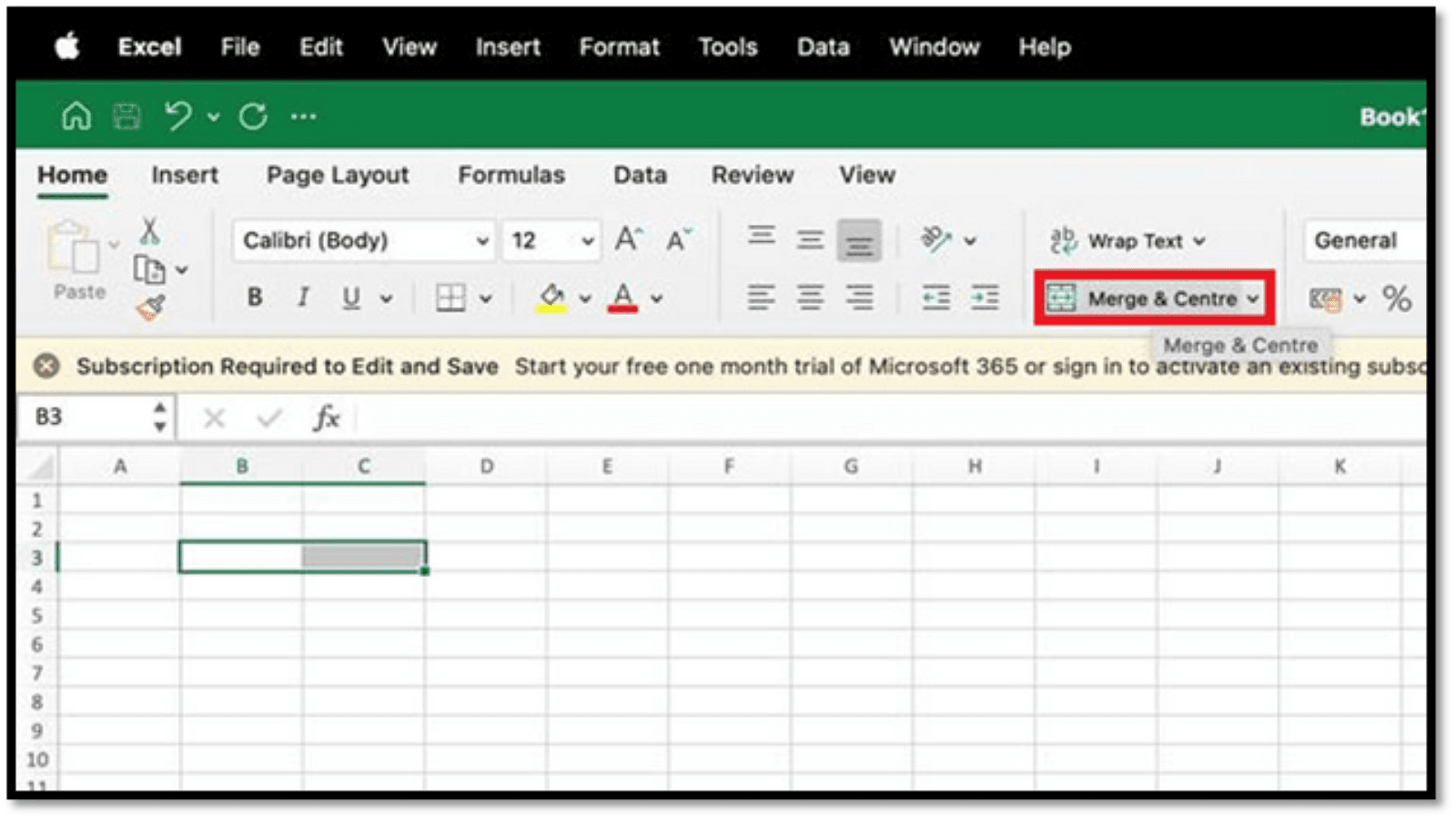
Next, navigate to the Home tab on the Excel ribbon at the top.
Step 3:
In the Home tab, locate the Merge & Center group. Just click on Merge Cells there.
And that's it! You've successfully merged your cells with just a few clicks. Easy, right?
Merging Cells in Excel Online
If you've got a Microsoft 365 plan or an Outlook account, you can easily use Excel Online. Here's how you can merge cells in just a few steps:
Step 1:
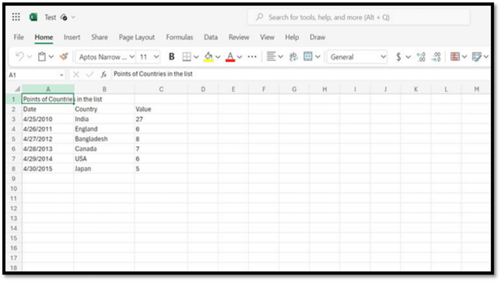
First, log in to your Microsoft Office 365 Online or Outlook account and open up the Excel Online worksheet you're working with.
Step 2:
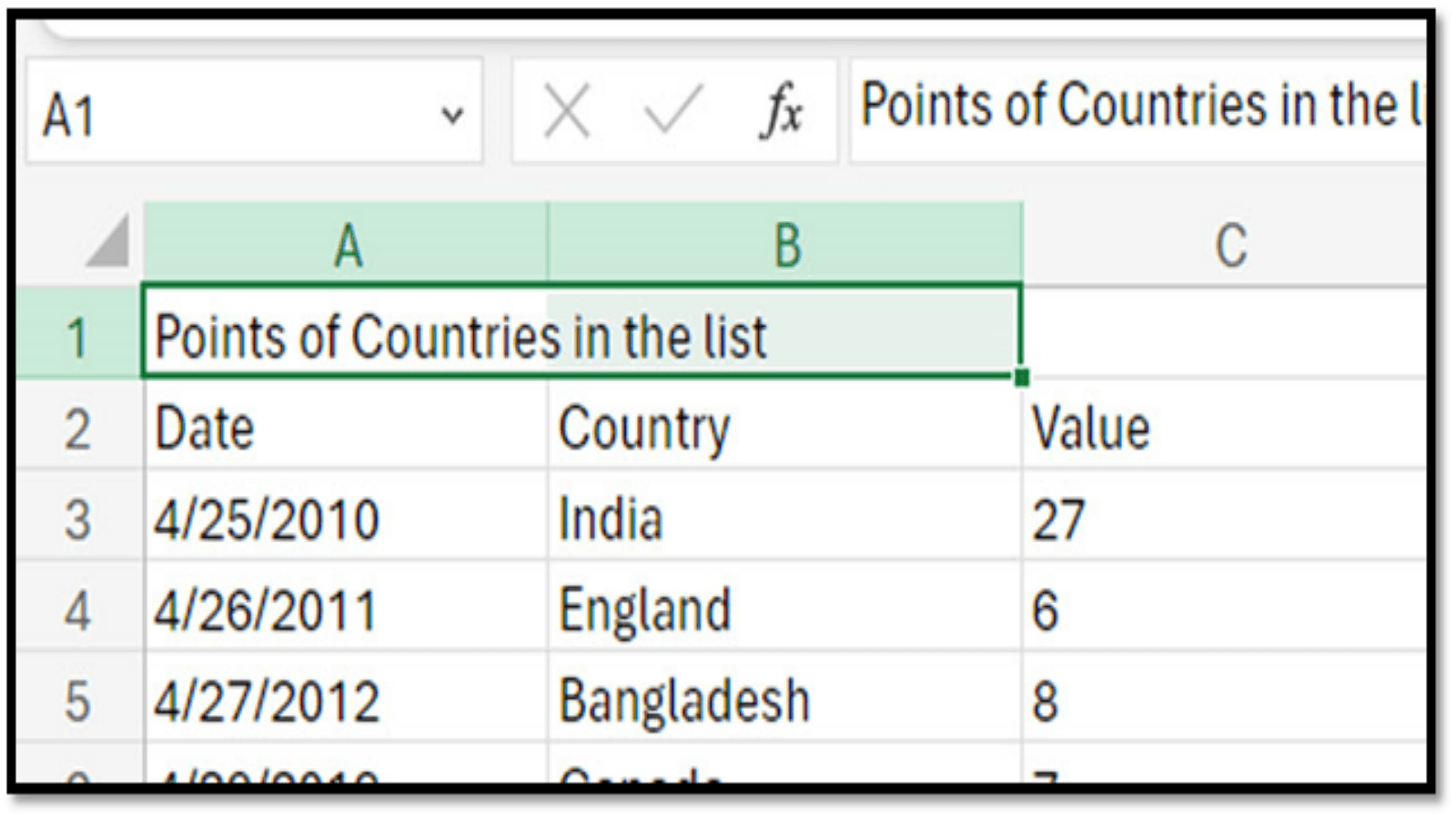
Then, go ahead and select the cells you're looking to merge.
Step 3:
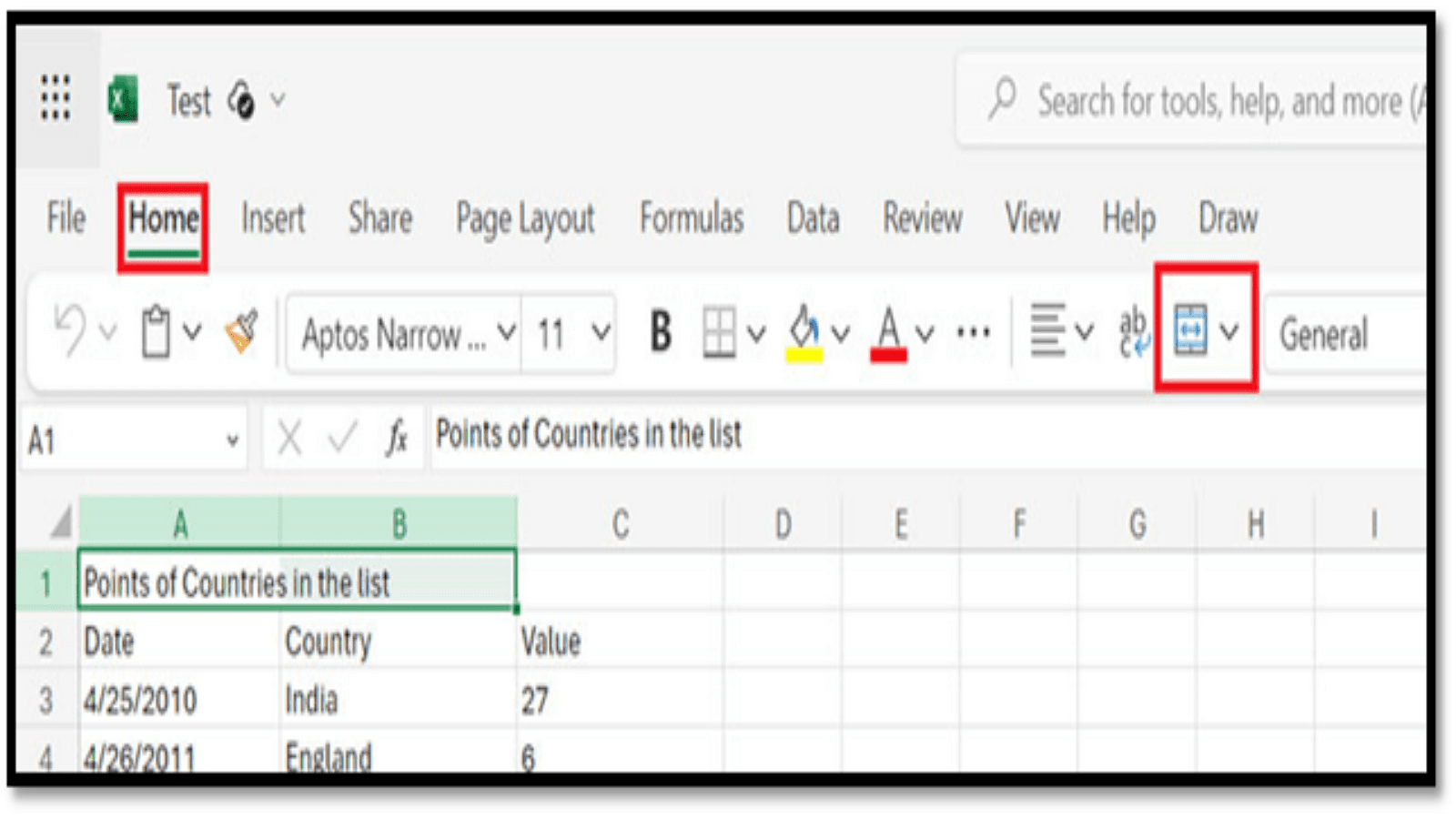
Navigate to the Home tab. There, you'll see the Merge Cells button—click it to automatically merge and center your selected cells.
Extra Tip
If you want more merging options, click on the dropdown button next to Merge Cells. You'll find a few different ways to merge, depending on what you need.
And there you have it—merging cells online is a breeze!
Merging Multiple Cells Without Losing Data
When you merge cells in Excel, only the content from one cell remains, and the rest gets deleted. So, you might be asking, "How can I merge multiple cells without losing any data?" Don't worry; I've got you covered. Two methods can help you do this: the CONCATENATE method and the ampersand (&) method.
Method 1. CONCATENATE Formula Method
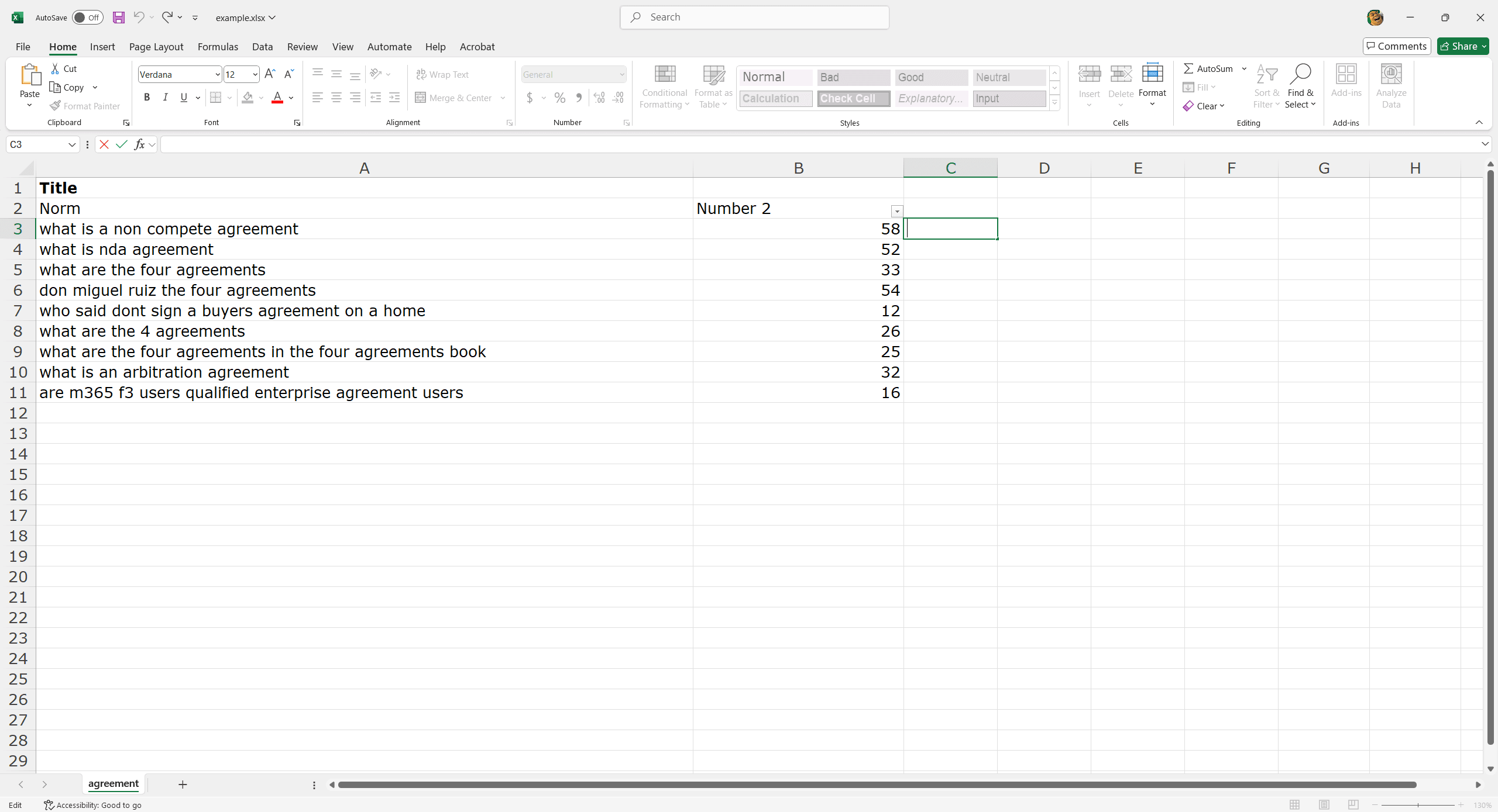
Step 1:
Choose the cell where you want your merged data to end up. Make sure this cell isn't part of the cells you're merging.
Step 2:
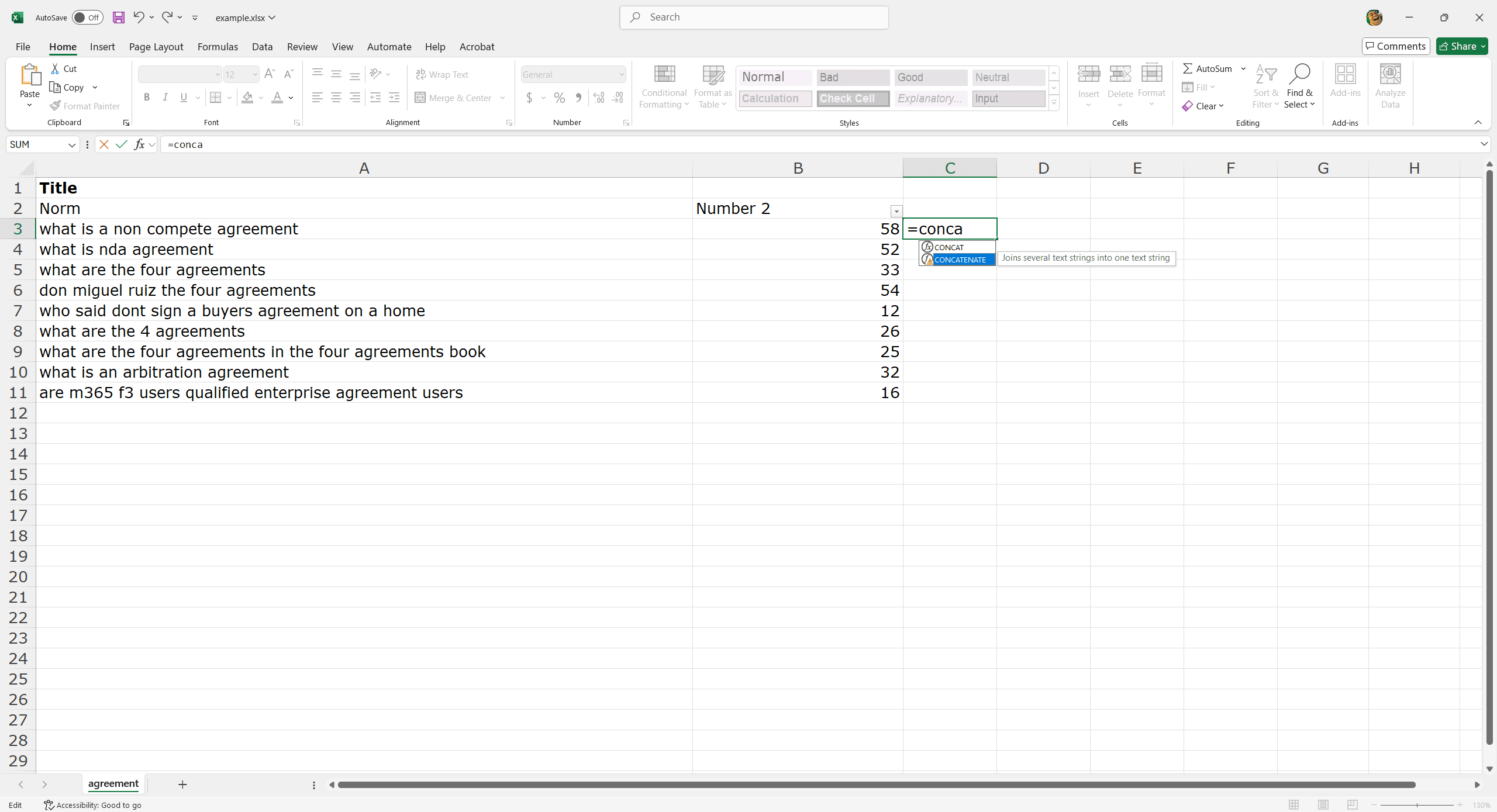
Type in the CONCATENATE formula in the selected cell. The basic structure of this formula is =CONCATENATE.
Step 3:
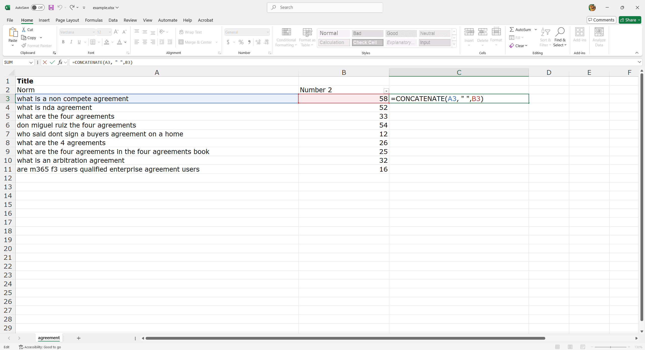
Select the cells with the data you want to merge. To add spaces between the merged values, use " " in your formula.
For example, your formula should look something like this: =CONCATENATE(A2, " ", B2).
Step 4:
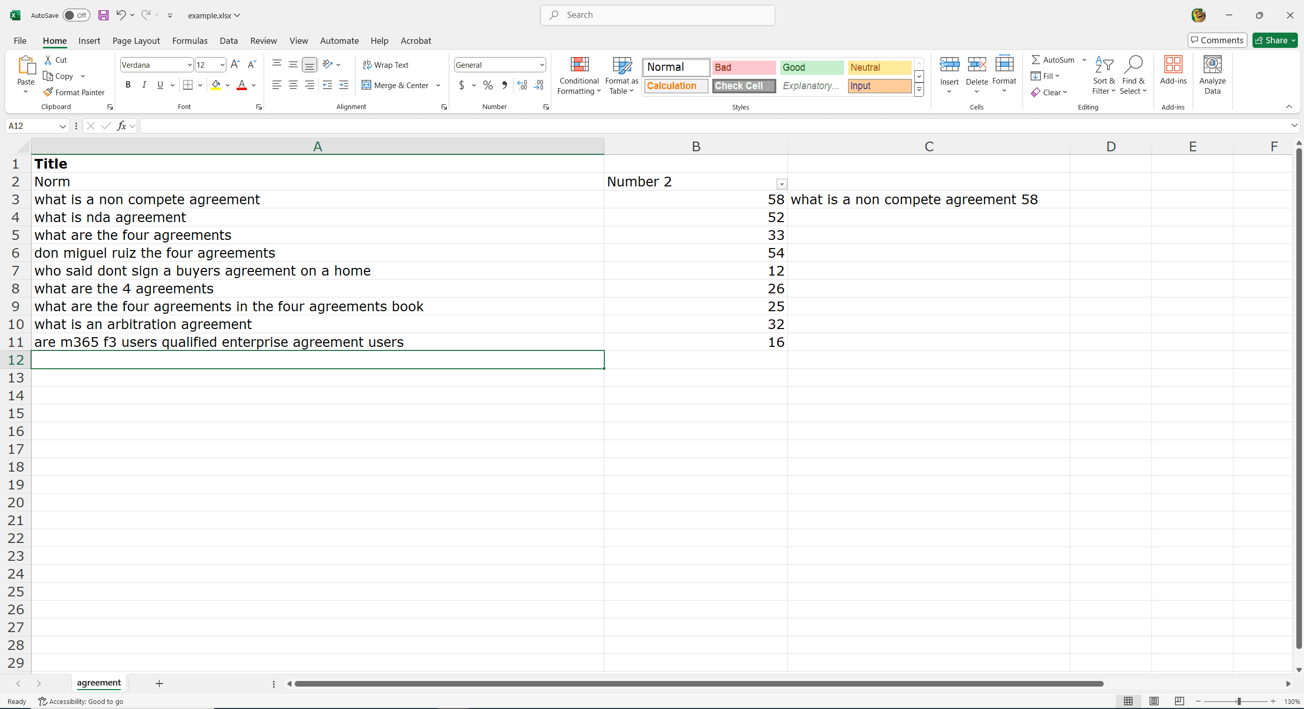
Hit Enter, and voilà! The content of the selected cells will merge into your formula cell.
Note:
To apply this formula to other cells, drag the fill handle (the tiny square at the bottom-right corner of the cell). This way, adjacent cells will be filled with the concatenated data.
Method 2. Ampersand (&) Method
Step 1:
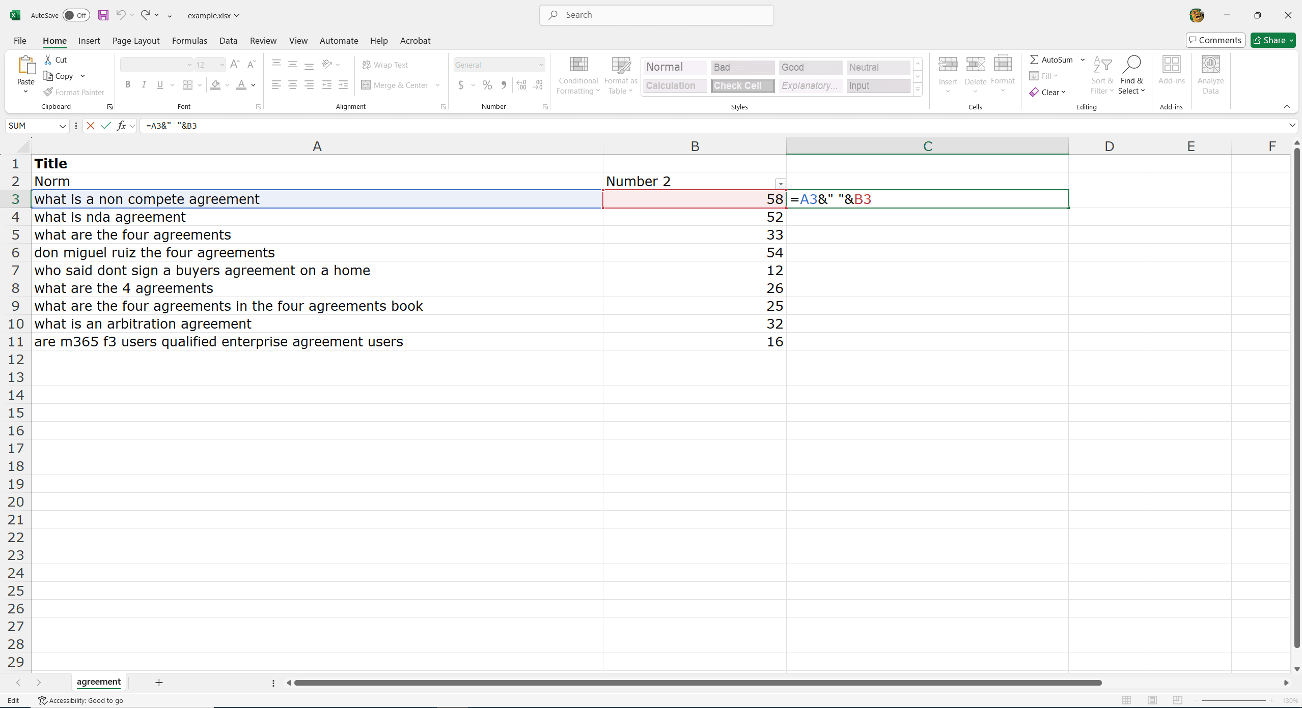
Type = in the cell where you want the merged data to appear.
Step 2:
Select the first cell to combine and type &. To add space between the data, type " " after the ampersand.
Step 3:
Select the second cell and then press Enter.
For example, your formula should look like this: =A2&" "&B2.
Step 4:
The data from the two cells will now be combined and shown in your selected cell.
Step 5:
To repeat this for other cells, click on the fill handle of the cell with your new value and drag it down. This will apply the same formula to adjacent cells.
And that's how you can merge cells without losing any data! Easy, right?
Using the TEXTJOIN Function for Lists
TEXTJOIN is a fantastic tool when you need to combine multiple cells and add a separator, like building a list of items.
Scenario:
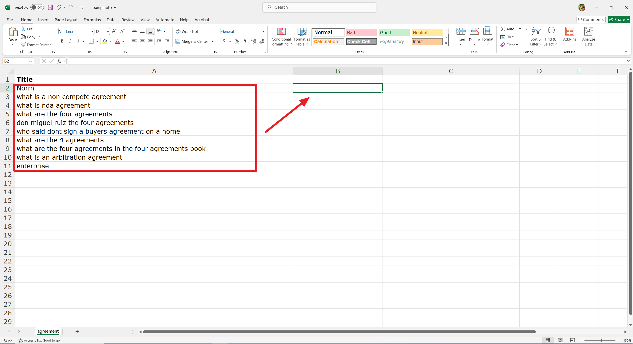
- Imagine you have a list of names in cells A2 to A7.
- You want to create a single cell, say B2, that lists all these names separated by commas.
Steps:
- Click on an empty cell where you want the combined data to appear, for example, B2.
- Use the TEXTJOIN function.
Here's how your formula should look if your names are in cells A2 through A7:
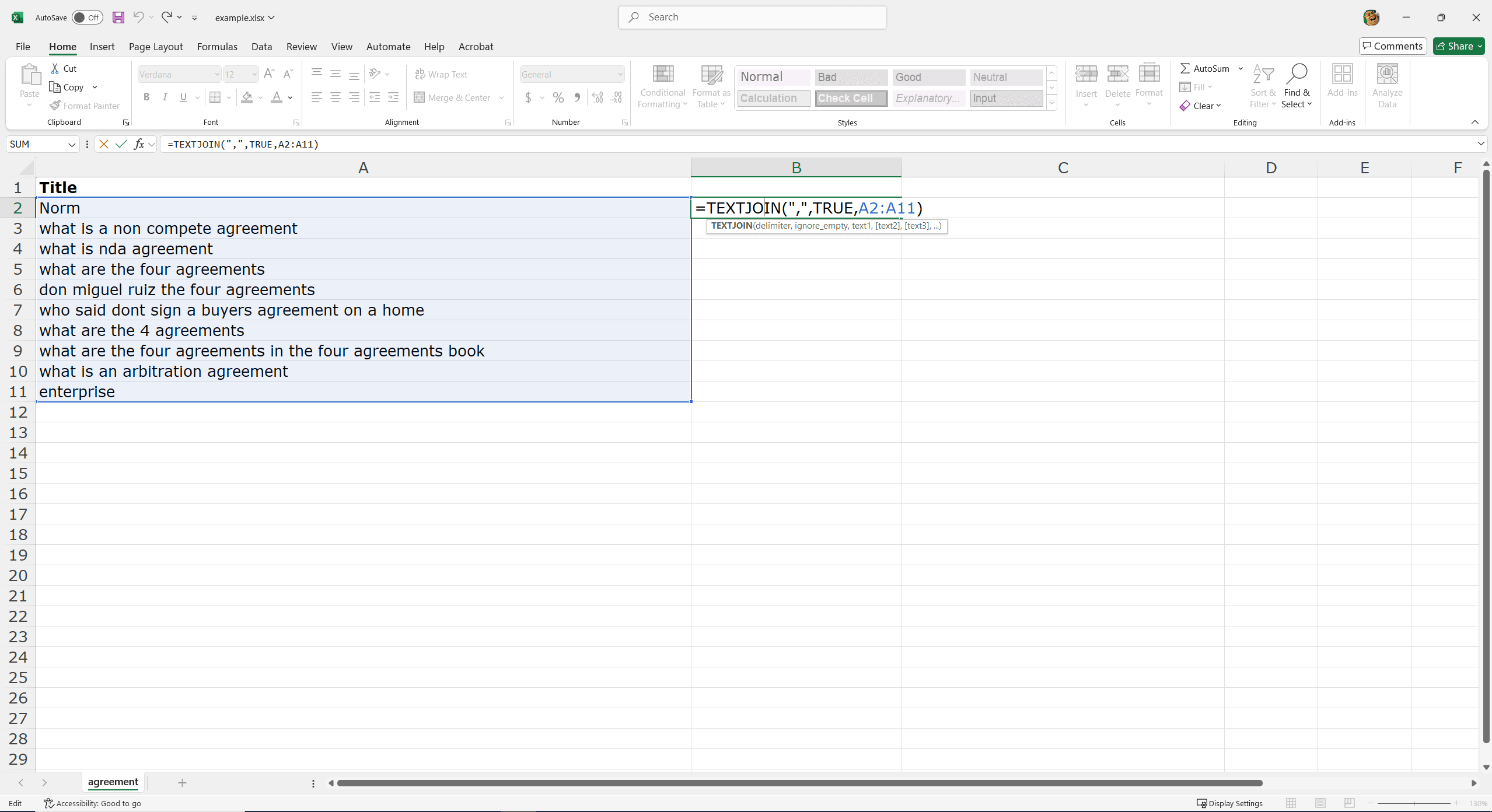
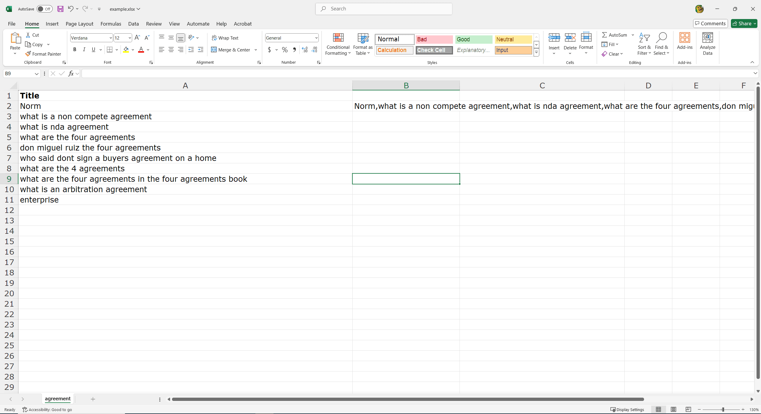
This formula will join all the names into one cell, with each name separated by a comma and a space.
And there you have it! All your names are neatly combined into one cell.
Final Words
And there you have it—several killer ways to merge cells in Excel without breaking a sweat. Whether you're consolidating names, making lists, or just want a cleaner look for your data, you've now got the tools and tricks to make it happen. With these methods—CONCATENATE, TEXTJOIN, and the trusty ampersand—you'll be whipping your spreadsheets into shape like a pro. Happy Excel-ing!

