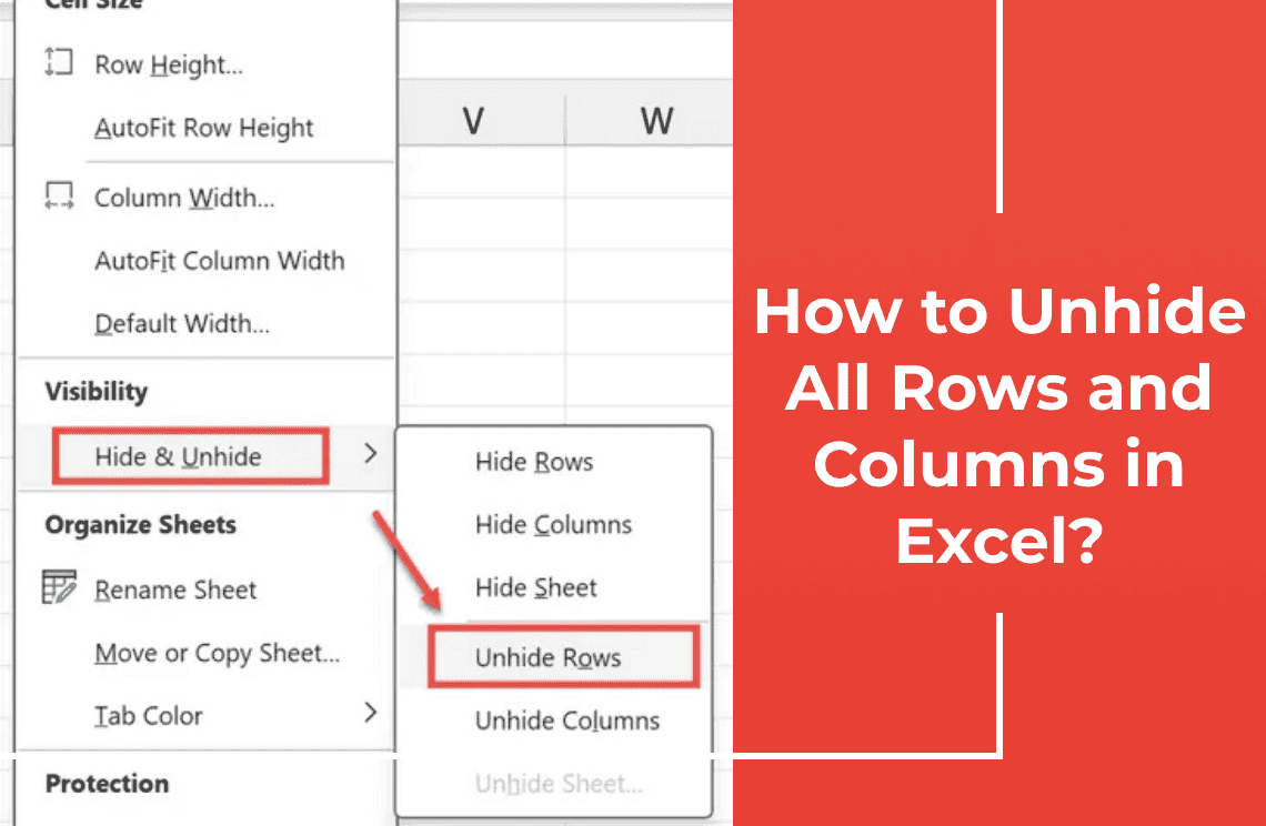
Hidden rows and columns got you stumped? No problem! This guide will show you how to unhide all your data in Excel quickly. Let's get your spreadsheet back to normal!
So, How to Unhide Rows in Excel with Quick and Easy Steps.
You open an Excel sheet and something doesn't look right. Maybe it is missing data or you suspect some hidden rows. Mostly it happens when working with shared documents. Now you want back your rows? Here are a few simple methods:
Option 1: Using the Ribbon Menu (The Visual Approach)
1. First, select the area where you think those hidden rows are hiding. You know, click and drag to highlight the range.
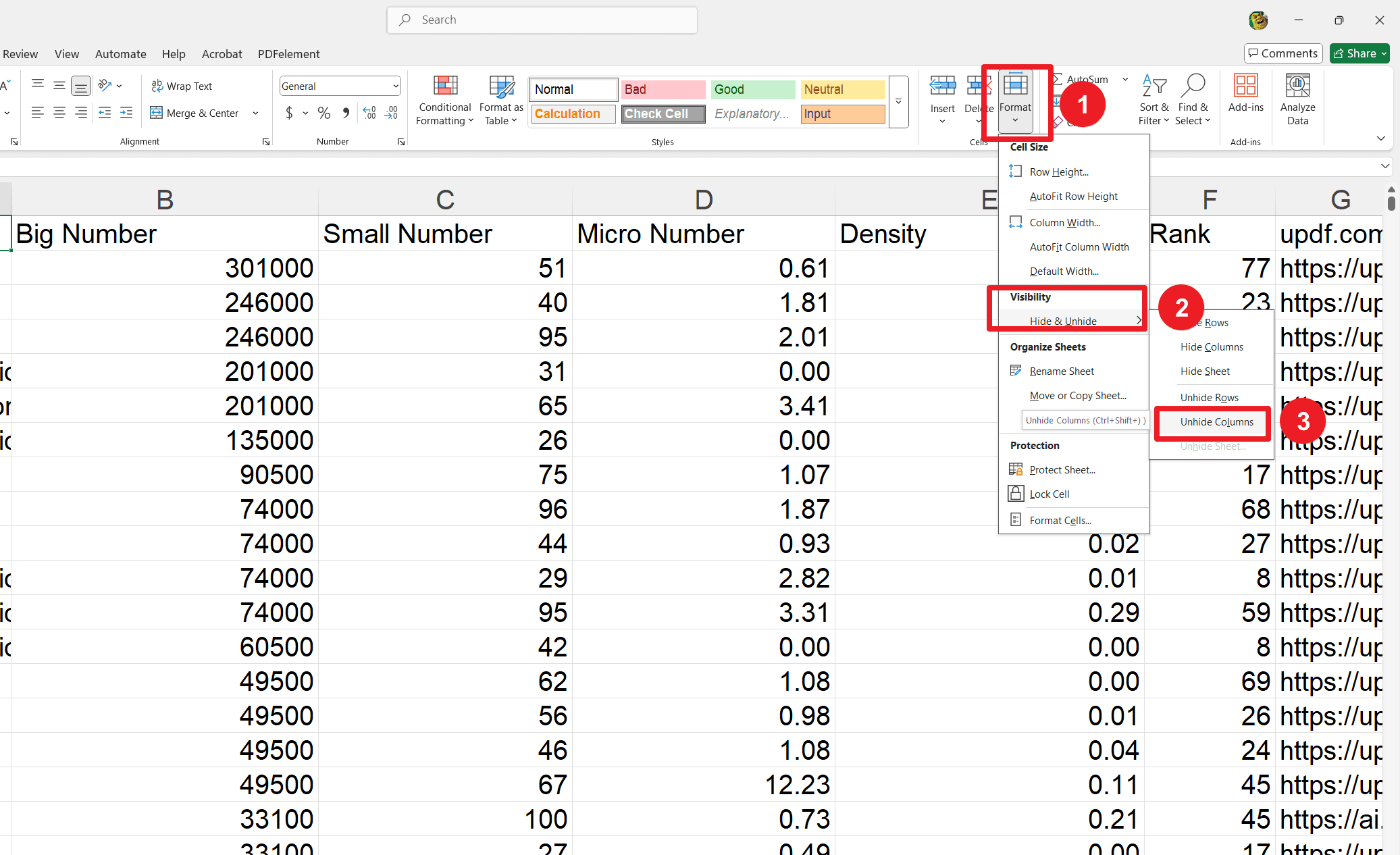
2. Now, head over to the 'Home' tab. You'll see the 'Format' button in the 'Cells' group. Go ahead and click that.
3. Hover your mouse over 'Hide & Unhide.' See it? Then, select 'Unhide Rows.' And just like that, hopefully, your rows will reappear.
Option 2: Using the Right-Click Context Menu (The Speedy Option)
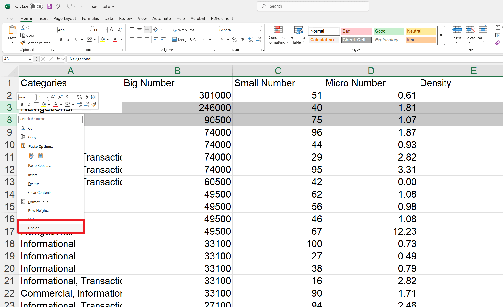
1. This one's even faster. Select the row numbers that include the hidden rows. Just click on the numbers on the left side of the sheet.
2. Right-click on the highlighted area. You know, the good old right-click.
3. Then, simply click 'Unhide' from the pop-up menu. So Easy.
Option 3: Using Keyboard Shortcuts (For the Keyboard Fans)
1. If you're a fan of shortcuts, this one's for you. Select the rows right above and below the hidden row(s). Get those rows highlighted.
2. Now, press Ctrl + Shift + 9. Hold those keys down together.
3. And boom! Your hidden rows should be back.
How to Unhide the First Row?
Ever opened an Excel sheet and noticed the first row is MIA? Yeah, it happens. And it can be a little frustrating, especially when you need that data. Don't worry, though! Here are some simple ways to bring that top row back into view.
Method 1: The Mouse Drag Trick (For When You're Feeling Visual)
1. Okay, first, look at those row numbers on the left. Find the very first row you can see. Let's say it's row 3. Click right on that number.
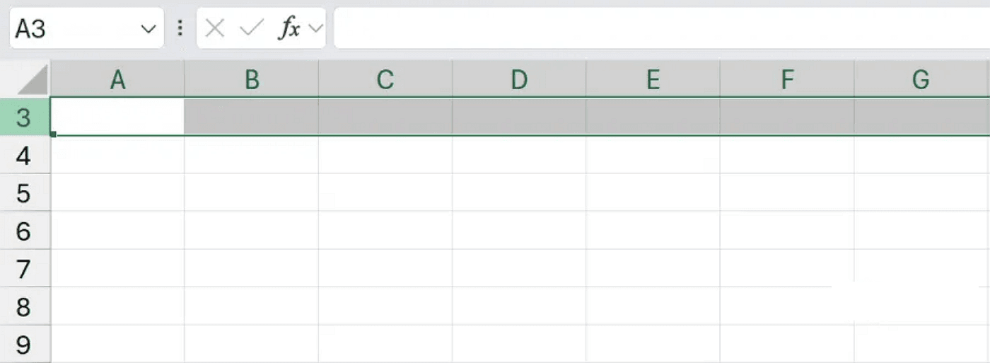
2. Now, here's the magic part. With that row still selected, hold your left mouse button down and drag your cursor upward. You're telling Excel, 'Hey, something is hiding up there, grab it too!'
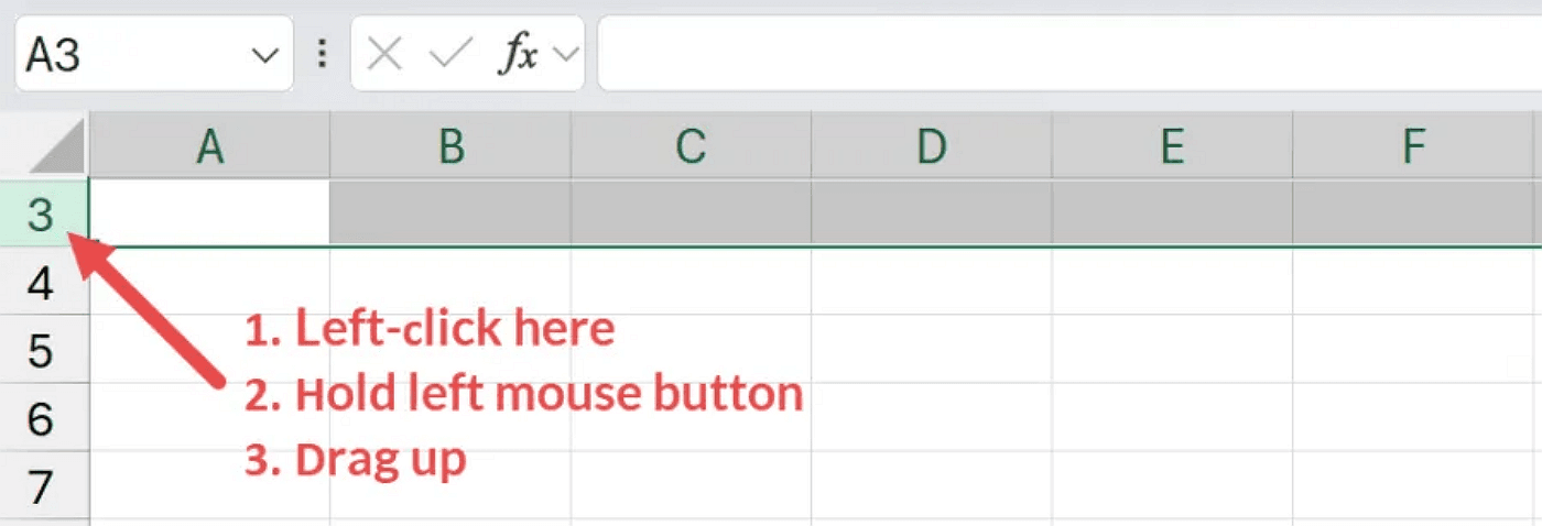
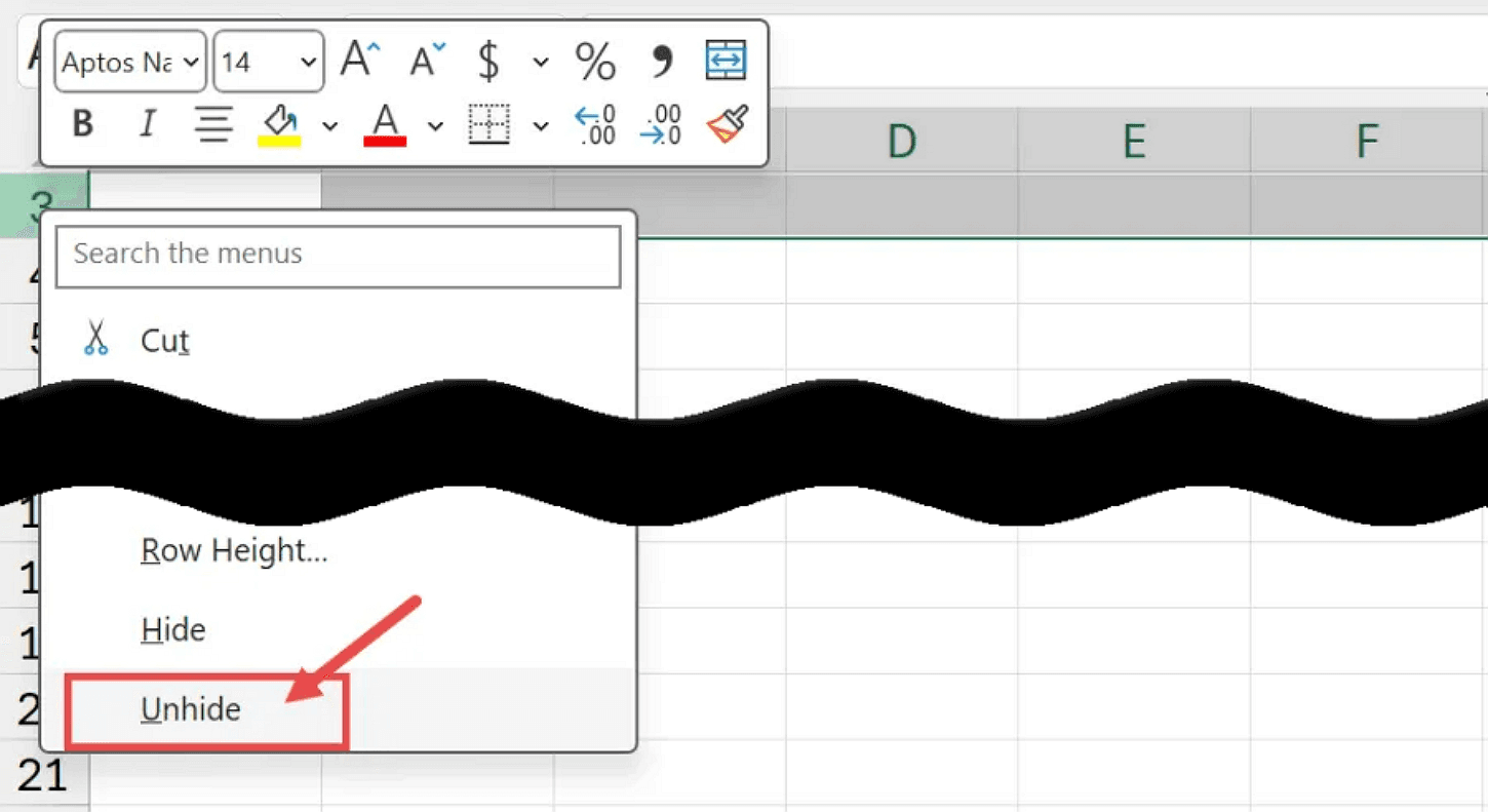
3. Then, just right-click on that first visible row again. See that 'Unhide' option? Click it! And just like that, row 1 should pop back into existence.
Method 2: The Name Box Shortcut (For Those Who Love a Quick Command)
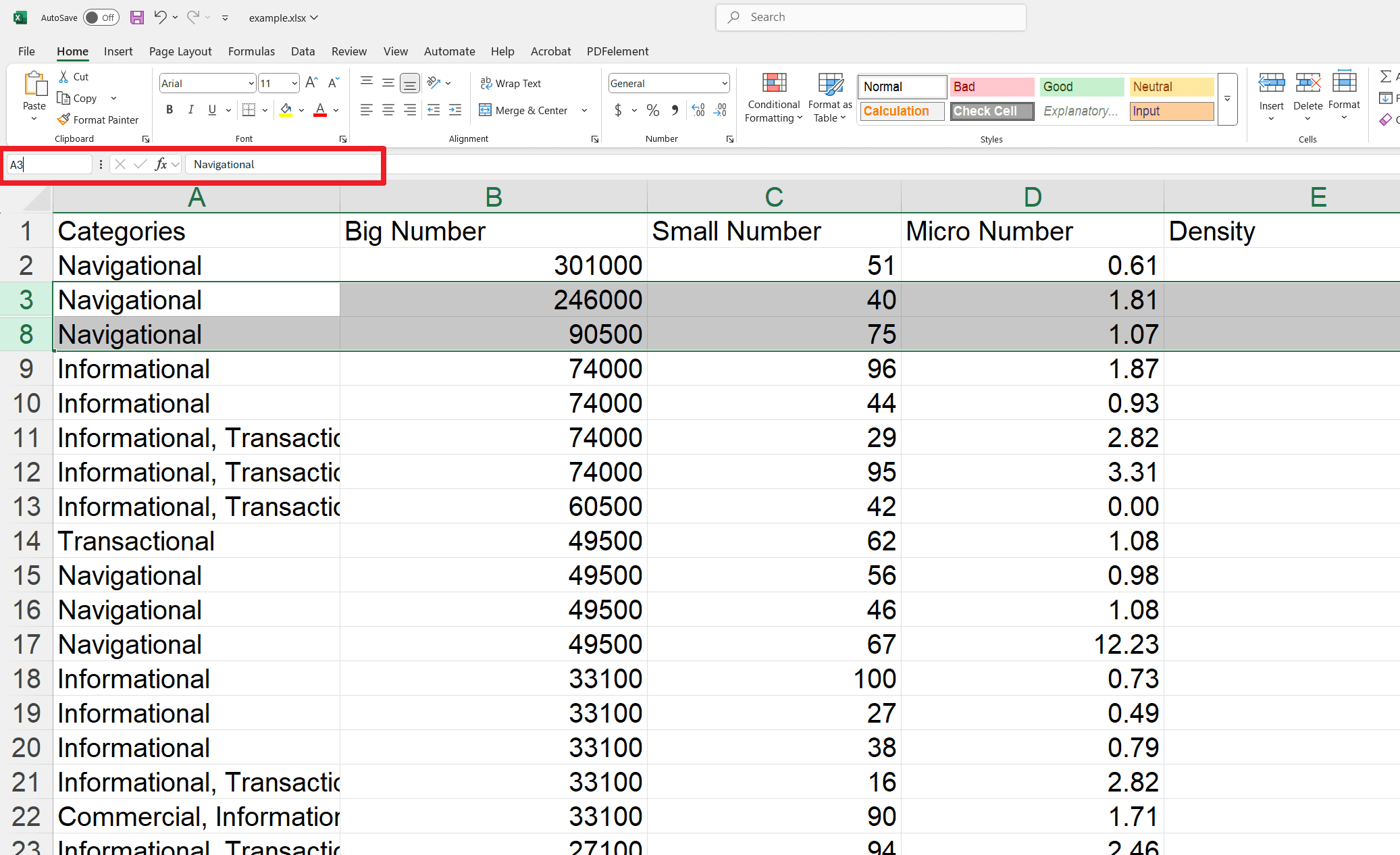
Step 1: Selecting the Hidden Row(s)
In the Name Box (next to the formula bar), type the range of the hidden rows. For example, 1:3 to select rows 1 through 3, and press Enter.
Step 2: Bringing Them Back!
1. Go to the Home tab.
2. Click Format in the Cells group.
3. Select Visibility > Hide & Unhide > Unhide Rows.
There you have it! Those hidden top rows don't stand a chance. Now, you can get back to your data without missing a beat.
How to Unhide All Rows in Excel?
To unhide all rows in an Excel sheet, follow these simple steps:
Step 1: Get Everything Selected (The Big Sweep!)
1. Click the Select All triangle in the top-left corner of the sheet, OR
2. Press Ctrl + A (press twice if needed to select the entire sheet).
Step 2: Time to Unhide! (Bring on the Light!)
Option 1 (Shortcut): Press Ctrl + Shift + 9.
Option 2 (Right-Click): Right-click anywhere on the selected sheet and select Unhide.
Option 3 (Ribbon): Go to the Home tab, click Format, and then select Unhide Rows.
How to Find Hidden Rows?
You can spot hidden rows by noticing gaps between row numbers. You can spot them if you're looking closely at the row numbers, but who has time for that when dealing with hundreds or thousands of rows? Don't worry; I've got a neat little trick to help you play detective and find those hidden lines quickly!
Step 1: Calling in the Special Ops (Go To Special!)
1. First things first, head over to the 'Home' tab. That's your command center for all things Excel.
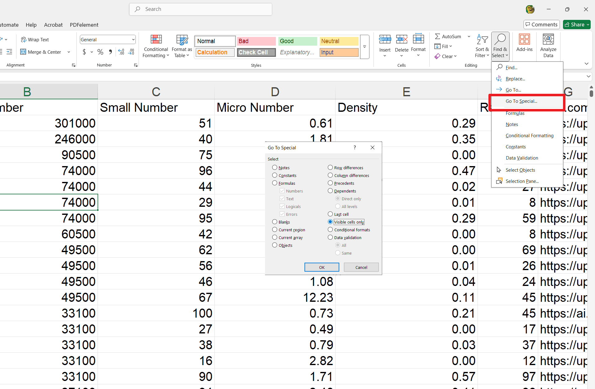
2. Now, look for the 'Editing' group. See that 'Find & Select' button? Click it, and then choose 'Go To Special...' It's like calling in the special ops for hidden rows.
3. Or, if you're a shortcut ninja, just press Ctrl + G. That'll bring up the 'Go To' dialog box. Then, click 'Special...' and you're on your way.
Step 2: Visible Cells Only - Your Secret Weapon!
1. You'll see many options once you're in the 'Go To Special' window. Look for 'Visible cells only' and give it a click. Then, hit 'OK'.
2. Here's the cool part: Excel will now highlight all the cells you can see. And get this – it'll mark the rows next to those hidden ones with a thin white border. It's like a secret code telling you, 'Hey, something's hiding here!' Now, you can easily spot where those hidden rows are lurking.
And there you have it! No more squinting at row numbers or scrolling endlessly. With this trick, you'll master finding hidden rows in no time.
Final Words
We hope this guide has helped you bring your hidden data to light! Now unhiding rows and columns is a quick fix that can save you a lot of hindrances. So, if you want to learn more about maximizing your Excel efficiency there are plenty more where that came from! Check out these useful resources:
More Excel tips here and More how-to and tips here. Keep exploring and keep learning!

