How to Use VLOOKUP in Excel Effortlessly?

Welcome, Excel enthusiasts! Have you ever found yourself lost in a sea of data and wished for a magic tool to retrieve information rapidly? You have to enter VLOOKUP, the Excel's hero in shining shield. This powerful function helps you search for specific values within your spreadsheets. Imagine finding a product price or employee information without scrolling through endless rows. Yes, VLOOKUP to the rescue! Let us dive into the wonders of VLOOKUP and break down its syntax. This guide also tackles common issues that come in using VLOOKUP. You will master the art of data management by the end of learning this. So, let us get started with its procedure!

What is the VLOOKUP Function in Excel?

Vertical Lookup or VLOOKUP is an Excel function. It searches for a value in the first column of a range and returns a corresponding value from another column in the same row at a time.

Usual Scenarios Where VLOOKUP Is Used

• Finding prices in a product list.
• Retrieving employee details.
• Matching invoice numbers with customer information.
• Looking up student grades or other academic records.

How VLOOKUP Can Streamline Data Retrieval?

• Efficient Data Management: It automates the retrieval process and avoid manual searches.
• Time-Saving: It quickly finds the information you need without scrolling through extensive spreadsheets.
• Error Minimization: It reduces the risk of manual errors in data management.
• Enhanced Data Accuracy: It ensures consistency and precision in data retrieval.

Users can manage their data more effectively and gain quick access to vital information by utilizing VLOOKUP.

VLOOKUP Formula Syntax

The VLOOKUP formula in Excel follows this structure:

• lookup_value: It is the value you want to find within the first column of your defined table range. It serves as the search key.
• table_array: It is the range of cells where VLOOKUP will search for the lookup_value. The first column in this range is where the function looks for the lookup_value. The rest are potential columns for data retrieval.
• col_index_num: A number representing the column in the table_array from which to return a value. If you want data from the third column, you would set this parameter to 3.
• [range_lookup]: An optional argument. Set to TRUE for an approximate match or FALSE for an exact match. When omitted, it defaults to TRUE. Using FALSE ensures you retrieve accurate, specific data.

So, How VLOOKUP Works?

1. Organize Your Data: Ensure your lookup values are in the first column of your data table.

2. Start the Formula: In the cell where you want the result, type =VLOOKUP(.

3. Specify the Lookup Value: Enter the value you're searching for (e.g., a cell reference like A2 or text like "Product123").

4. Define the Table: Select the range of cells containing your data, including the lookup column and the result column(s).

5. Set the Column Number: Enter the column number (counting from the first column of your selected table) that contains the result you want.

6. Choose Match Type: Type FALSE for an exact match or TRUE (or leave blank) for an approximate match.

7. Finish and Check: Close with ")" and press Enter. Verify the result and troubleshoot any errors like #N/A by checking your lookup value, table range, and match type.

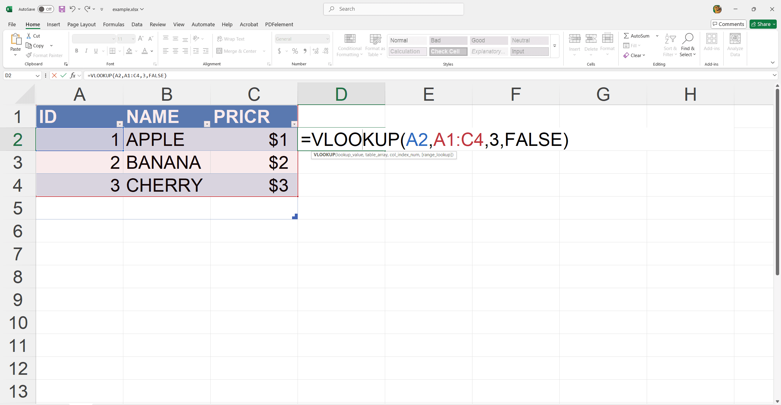
Practical Example For Managing Inventory Data with VLOOKUP

Think of managing an inventory list with a spreadsheet where each product has a unique ID alongside columns for product name and cost. Use VLOOKUP to find the cost of a product using its ID.

1. Setup: Have your product data organized? For example, columns A to C respectively for ID, name, and price.

2. Formula: Use a VLOOKUP formula like =VLOOKUP(E2, A2:C20, 3, FALSE).

• Here, E2 contains the product ID you're searching for.
• A2:C20 is the table array where your data resides.
• 3 specifies the column index for price.
• FALSE ensures an exact match.

By executing this, you quickly retrieve the price, optimizing inventory management efficiently without constant manual data checks.

Advanced Usage: VLOOKUP Between Two Sheets

1. Setup: Suppose Sheet1 has an Employee ID list and Sheet2 contains IDs and contact information.

2. Identify Cell: In Sheet 1, identify the cell with the Employee ID. For example, A2.

3. Formula: Use the formula: =VLOOKUP(A2, Sheet2!A2:C100, 3, FALSE) on Sheet1

• Sheet2!A2:C100 specifies the range in Sheet2 to search.
• 3 refers to the column index containing contact details.
• FALSE ensures an exact match.

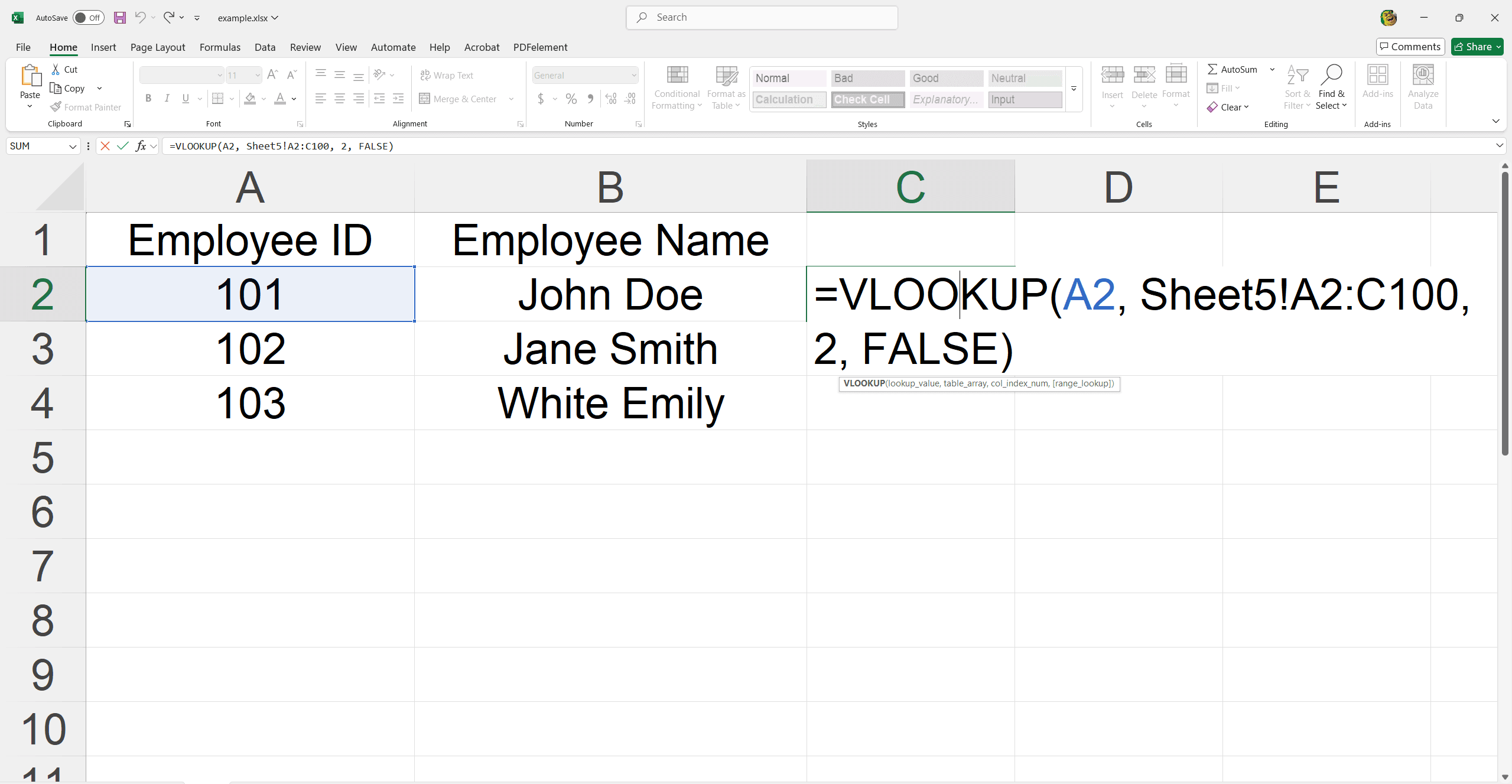
4. Execute: Press Enter to retrieve the contact details seamlessly across sheets.

Step-by-Step Solution

1. Setup VLOOKUP in the First Sheet: Identify the cell with the lookup value, e.g., A2.

2. Use VLOOKUP Formula: Example: =VLOOKUP(A2, Sheet2!A2:C100, 3, FALSE).

3. Copy Formula to Multiple Rows: Drag the fill handle down to apply to other rows.

4. Verify Results: Ensure the data returned is accurate for each row.

Using VLOOKUP Between Two Workbooks

VLOOKUP can reference data across different workbooks. It facilitates seamless data integration and uniformity. It is beneficial for managing large datasets spread across multiple documents.

Linking Sales Data:

1. Formula: Suppose Workbook1.xlsx contains sales IDs and Workbook2.xlsx holds detailed sales data.
2. Setup in Workbook1.xlsx: Use =VLOOKUP(A2, '[Workbook2.xlsx]Sheet1'!$A$2:$D$100, 4, FALSE).

• A2 is the lookup value in Workbook1.xlsx.
• '[Workbook2.xlsx]Sheet1'!$A$2:$D$100 is the range in Workbook2.xlsx.
• 4 specifies the column index for the desired data.

1. Execute and Verify: This returns the relevant sales data, ensuring comprehensive data management across workbooks.

Step-by-Step Guide

1. Launch Both Workbooks: Launch Workbook1.xlsx and Workbook2.xlsx.

2. Set Up VLOOKUP: In Workbook1.xlsx, enter: =VLOOKUP(A2, '[Workbook2.xlsx]Sheet1'!$A$2:$D$100, 4, FALSE).

3. Enter and Copy Formula: Drag the formula to apply to other rows.

4. Ensure Accuracy and Troubleshooting: Verify data.

5. Check for errors like #N/A or wrong range references in sheet.

Common Issues and Troubleshooting Solutions

Handling #N/A Errors:

#N/A typically appears if the lookup value isn't in the range. So, double check the value and ensure it exists in the referenced sheet.

Checking for Data Inconsistencies:

Ensure that the lookup value and the reference column match the data types. Text in one and number in the other can cause issues. And, remove any leading or trailing spaces that might cause mismatches.

Defining Data Ranges Accurately:

When copying formulas, use absolute references (e.g., $A$2:$D$100) to keep the range constant. It ensures the range covers all necessary rows and columns to capture your data accurately.

For Further Reading

That's it! You've got the basics of using VLOOKUP down. Do not worry if you run into issues like #N/A errors or data mismatches. Practice makes perfection. The more you use VLOOKUP the better you will get at spotting and fixing these glitches.

Now take some time to experiment and get comfortable with this powerful gizmo. Check out Excel Tips and How-To and Tips for more great tips and tricks. Keep practicing and soon enough, you'll be an Excel wizard! Happy spreadsheeting!